Greene W.H. Econometric Analysis

Подождите немного. Документ загружается.

CHAPTER 3

✦

Least Squares

variable. Show that replacing missing values of x with the mean of the complete

observations has the same effect as adding the new variable.

7. Demand system estimation. Let Y denote total expenditure on consumer durables,

nondurables, and services and E

, E

, and E

are the expenditures on the three

categories. As deﬁned, Y = E

+ E

. Now, consider the expenditure system

= α

+ β

Y + γ

+ γ

+ ε

= α

+ β

Y + γ

+ γ

+ ε

= α

+ β

Y + γ

+ γ

+ ε

Prove that if all equations are estimated by ordinary least squares, then the sum

of the expenditure coefﬁcients will be 1 and the four other column sums in the

preceding model will be zero.

8. Change in adjusted R

. Prove that the adjusted R

in (3-30) rises (falls) when

variable x

is deleted from the regression if the square of the t ratio on x

in the

multiple regression is less (greater) than 1.

9. Regression without a constant. Suppose that you estimate a multiple regression ﬁrst

with, then without, a constant. Whether the R

is higher in the second case than

the ﬁrst will depend in part on how it is computed. Using the (relatively) standard

method R

= 1 − (e



e/y



y), which regression will have a higher R

10. Three variables, N, D, and Y, all have zero means and unit variances. A fourth

variable is C = N + D. In the regression of C on Y, the slope is 0.8. In the regression

of C on N, the slope is 0.5. In the regression of D on Y, the slope is 0.4. What is the

sum of squared residuals in the regression of C on D? There are 21 observations

and all moments are computed using 1/(n − 1) as the divisor.

11. Using the matrices of sums of squares and cross products immediately preceding

Section 3.2.3, compute the coefﬁcients in the multiple regression of real investment

on a constant, real GNP and the interest rate. Compute R

12. In the December 1969, American Economic Review (pp. 886–896), Nathaniel Leff

reports the following least squares regression results for a cross section study of the

effect of age composition on savings in 74 countries in 1964:

ln S/Y = 7.3439 + 0.1596 ln Y/N +0.0254 ln G − 1.3520 ln D

− 0.3990 ln D

ln S/N = 2.7851 + 1.1486 ln Y/N + 0.0265 ln G − 1.3438 ln D

− 0.3966 ln D

where S/Y = domestic savings ratio, S/N = per capita savings, Y/N = per capita

income, D

=percentage of the population under 15, D

=percentage of the popu-

lation over 64, and G = growth rate of per capita income. Are these results correct?

Explain. [See Goldberger (1973) and Leff (1973) for discussion.]

Application

The data listed in Table 3.5 are extracted from Koop and Tobias’s (2004) study of

the relationship between wages and education, ability, and family characteristics. (See

Appendix Table F3.2.) Their data set is a panel of 2,178 individuals with a total of 17,919

observations. Shown in the table are the ﬁrst year and the time-invariant variables for

the ﬁrst 15 individuals in the sample. The variables are deﬁned in the article.

PART I

✦

The Linear Regression Model

TABLE 3.5

Subsample from Koop and Tobias Data

Mother’s Father’s

Person Education Wage Experience Ability education education Siblings

1 13 1.82 1 1.00 12 12 1

2 15 2.14 4 1.50 12 12 1

3 10 1.56 1 −0.36 12 12 1

4 12 1.85 1 0.26 12 10 4

5 15 2.41 2 0.30 12 12 1

6 15 1.83 2 0.44 12 16 2

7 15 1.78 3 0.91 12 12 1

8 13 2.12 4 0.51 12 15 2

9 13 1.95 2 0.86 12 12 2

10 11 2.19 5 0.26 12 12 2

11 12 2.44 1 1.82 16 17 2

12 13 2.41 4 −1.30 13 12 5

13 12 2.07 3 −0.63 12 12 4

14 12 2.20 6 −0.36 10 12 2

15 12 2.12 3 0.28 10 12 3

Let X

equal a constant, education, experience, and ability (the individual’s own

characteristics). Let X

contain the mother’s education, the father’s education, and the

number of siblings (the household characteristics). Let y be the wage.

a. Compute the least squares regression coefﬁcients in the regression of y on X

Report the coefﬁcients.

b. Compute the least squares regression coefﬁcients in the regression of y on X

and

. Report the coefﬁcients.

c. Regress each of the three variables in X

on all the variables in X

. These new

variables are X

∗

. What are the sample means of these three variables? Explain the

ﬁnding.

d. Using (3-26), compute the R

for the regression of y on X

and X

. Repeat the

computation for the case in which the constant term is omitted from X

. What

happens to R

e. Compute the adjusted R

for the full regression including the constant term. Inter-

pret your result.

f. Referring to the result in part c, regress y on X

and X

∗

. How do your results

compare to the results of the regression of y on X

and X

? The comparison you

are making is between the least squares coefﬁcients when y is regressed on X

and

and when y is regressed on X

and X

. Derive the result theoretically. (Your

numerical results should match the theory, of course.)

THE LEAST SQUARES

ESTIMATOR

4.1 INTRODUCTION

Chapter 3 treated ﬁtting the linear regression to the data by least squares as a purely

algebraic exercise. In this chapter, we will examine in detail least squares as an estimator

of the model parameters of the linear regression model (deﬁned in Table 4.1). We begin

in Section 4.2 by returning to the question raised but not answered in Footnote 1,

Chapter 3—that is, why should we use least squares? We will then analyze the estimator

in detail. There are other candidates for estimating β. For example, we might use the

coefﬁcients that minimize the sum of absolute values of the residuals. The question of

which estimator to choose is based on the statistical properties of the candidates, such

as unbiasedness, consistency, efﬁciency, and their sampling distributions. Section 4.3

considers ﬁnite-sample properties such as unbiasedness. The ﬁnite-sample properties

of the least squares estimator are independent of the sample size. The linear model is

one of relatively few settings in which deﬁnite statements can be made about the exact

ﬁnite-sample properties of any estimator. In most cases, the only known properties

are those that apply to large samples. Here, we can only approximate ﬁnite-sample

behavior by using what we know about large-sample properties. Thus, in Section 4.4,

we will examine the large-sample or asymptotic properties of the least squares estimator

of the regression model.

Discussions of the properties of an estimator are largely concerned with point

estimation—that is, in how to use the sample information as effectively as possible to

produce the best single estimate of the model parameters. Interval estimation, con-

sidered in Section 4.5, is concerned with computing estimates that make explicit the

uncertainty inherent in using randomly sampled data to estimate population quanti-

ties. We will consider some applications of interval estimation of parameters and some

functions of parameters in Section 4.5. One of the most familiar applications of interval

estimation is in using the model to predict the dependent variable and to provide a

plausible range of uncertainty for that prediction. Section 4.6 considers prediction and

forecasting using the estimated regression model.

The analysis assumes that the data in hand correspond to the assumptions of the

model. In Section 4.7, we consider several practical problems that arise in analyzing

nonexperimental data. Assumption A2, full rank of X, is taken as a given. As we noted

in Section 2.3.2, when this assumption is not met, the model is not estimable, regardless

of the sample size. Multicollinearity, the near failure of this assumption in real-world

This discussion will use our results on asymptotic distributions. It may be helpful to review Appendix D

before proceeding to this material.

PART I

✦

The Linear Regression Model

TABLE 4.1

Assumptions of the Classical Linear Regression Model

A1. Linearity: y

= x

+ x

+···+x

+ ε

A2. Full rank: The n × K sample data matrix, X, has full column rank.

A3. Exogeneity of the independent variables: E [ε

, x

,...,x

] = 0, i, j = 1,...,n.

There is no correlation between the disturbances and the independent variables.

A4. Homoscedasticity and nonautocorrelation: Each disturbance, ε

, has the same ﬁnite

variance, σ

, and is uncorrelated with every other disturbance, ε

, conditioned on X.

A5. Stochastic or nonstochastic data: (x

, x

,...,x

) i = 1,...,n.

A6. Normal distribution: The disturbances are normally distributed.

data, is examined in Sections 4.7.1 to 4.7.3. Missing data have the potential to derail

the entire analysis. The benign case in which missing values are simply manageable

random gaps in the data set is considered in Section 4.7.4. The more complicated case

of nonrandomly missing data is discussed in Chapter 18. Finally, the problem of badly

measured data is examined in Section 4.7.5.

4.2 MOTIVATING LEAST SQUARES

Ease of computation is one reason that least squares is so popular. However, there are

several other justiﬁcations for this technique. First, least squares is a natural approach

to estimation, which makes explicit use of the structure of the model as laid out in the

assumptions. Second, even if the true model is not a linear regression, the regression

line ﬁt by least squares is an optimal linear predictor for the dependent variable. Thus, it

enjoys a sort of robustness that other estimators do not. Finally, under the very speciﬁc

assumptions of the classical model, by one reasonable criterion, least squares will be

the most efﬁcient use of the data. We will consider each of these in turn.

4.2.1 THE POPULATION ORTHOGONALITY CONDITIONS

Let x denote the vector of independent variables in the population regression model and

for the moment, based on assumption A5, the data may be stochastic or nonstochas-

tic. Assumption A3 states that the disturbances in the population are stochastically

orthogonal to the independent variables in the model; that is, E [ε |x] =0. It follows that

Cov[x,ε] =0. Since (by the law of iterated expectations—Theorem B.1) E

{E [ε |x]}=

E [ε] = 0, we may write this as

[xε] = E

[x(y −x



β)] = 0

[xy] = E

[xx



]β. (4-1)

(The right-hand side is not a function of y so the expectation is taken only over x.) Now,

recall the least squares normal equations, X



y = X



Xb. Divide this by n and write it as

a summation to obtain





i=1







i=1





b. (4-2)

CHAPTER 4

✦

The Least Squares Estimator

Equation (4-1) is a population relationship. Equation (4-2) is a sample analog. Assuming

the conditions underlying the laws of large numbers presented in Appendix D are

met, the sums on the left-hand and right-hand sides of (4-2) are estimators of their

counterparts in (4-1). Thus, by using least squares, we are mimicking in the sample the

relationship in the population. We’ll return to this approach to estimation in Chapters 12

and 13 under the subject of GMM estimation.

4.2.2 MINIMUM MEAN SQUARED ERROR PREDICTOR

As an alternative approach, consider the problem of ﬁnding an optimal linear predictor

for y. Once again, ignore Assumption A6 and, in addition, drop Assumption A1 that

the conditional mean function, E [y |x] is linear. For the criterion, we will use the mean

squared error rule, so we seek the minimum mean squared error linear predictor of y,

which we’ll denote x



γ . The expected squared error of this predictor is

MSE = E

[y −x



γ ]

This can be written as

MSE = E

y,x



y − E [y |x]



+ E

y,x



E [y |x] − x





We seek the γ that minimizes this expectation. The ﬁrst term is not a function of γ ,so

only the second term needs to be minimized. Note that this term is not a function of y,

so the outer expectation is actually superﬂuous. But, we will need it shortly, so we will

carry it for the present. The necessary condition is

∂ E



[E(y |x) − x



γ ]



∂γ

= E



∂[E(y |x) − x



γ ]

∂γ



=−2E



x[E(y |x) − x



γ ]



=0.

Note that we have interchanged the operations of expectation and differentiation in

the middle step, since the range of integration is not a function of γ . Finally, we have

the equivalent condition

[xE(y |x)] = E

[xx



]γ .

The left-hand side of this result is E

[xE(y |x)] =Cov[x, E(y |x)] +E [x]E

[E(y |x)] =

Cov[x, y] + E [x]E [y] = E

[xy]. (We have used Theorem B.2.) Therefore, the nec-

essary condition for ﬁnding the minimum MSE predictor is

[xy] = E

[xx



]γ . (4-3)

This is the same as (4-1), which takes us to the least squares condition once again.

Assuming that these expectations exist, they would be estimated by the sums in

(4-2), which means that regardless of the form of the conditional mean, least squares

is an estimator of the coefﬁcients of the minimum expected mean squared error lin-

ear predictor. We have yet to establish the conditions necessary for the if part of the

theorem, but this is an opportune time to make it explicit:

PART I

✦

The Linear Regression Model

THEOREM 4.1

Minimum Mean Squared Error Predictor

If the data generating mechanism generating (x

, y

)

i=1,...,n

is such that the law of

large numbers applies to the estimators in (4-2) of the matrices in (4-1), then the

minimum expected squared error linear predictor of y

is estimated by the least

squares regression line.

4.2.3 MINIMUM VARIANCE LINEAR UNBIASED ESTIMATION

Finally, consider the problem of ﬁnding a linear unbiased estimator. If we seek the one

that has smallest variance, we will be led once again to least squares. This proposition

will be proved in Section 4.3.5.

The preceding does not assert that no other competing estimator would ever be

preferable to least squares. We have restricted attention to linear estimators. The pre-

ceding result precludes what might be an acceptably biased estimator. And, of course,

the assumptions of the model might themselves not be valid. Although A5 and A6 are

ultimately of minor consequence, the failure of any of the ﬁrst four assumptions would

make least squares much less attractive than we have suggested here.

4.3 FINITE SAMPLE PROPERTIES

OF LEAST SQUARES

An “estimator” is a strategy, or formula for using the sample data that are drawn from a

population. The “properties” of that estimator are a description of how that estimator

can be expected to behave when it is applied to a sample of data. To consider an

example, the concept of unbiasedness implies that “on average” an estimator (strategy)

will correctly estimate the parameter in question; it will not be systematically too high

or too low. It seems less than obvious how one could know this if they were only going

to draw a single sample of data from the population and analyze that one sample.

The argument adopted in classical econometrics is provided by the sampling properties

of the estimation strategy. A conceptual experiment lies behind the description. One

imagines “repeated sampling” from the population and characterizes the behavior of

the “sample of samples.” The underlying statistical theory of the the estimator provides

the basis of the description. Example 4.1 illustrates.

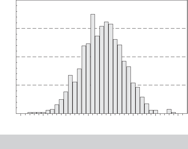
Example 4.1 The Sampling Distribution of a Least Squares Estimator

The following sampling experiment shows the nature of a sampling distribution and the

implication of unbiasedness. We drew two samples of 10,000 random draws on variables

and x

from the standard normal population (mean zero, variance 1). We generated a

set of ε

’s equal to 0.5w

and then y

= 0.5 + 0.5x

+ ε

. We take this to be our popula-

tion. We then drew 1,000 random samples of 100 observations on (y

, x

) from this popu-

lation, and with each one, computed the least squares slope, using at replication r , b





100

j =1

( x

− ¯x

) y







100

j =1

( x

− ¯x

)



. The histogram in Figure 4.1 shows the result of the ex-

periment. Note that the distribution of slopes has a mean roughly equal to the “true value”

of 0.5, and it has a substantial variance, reﬂecting the fact that the regression slope, like any

other statistic computed from the sample, is a random variable. The concept of unbiasedness

CHAPTER 4

✦

The Least Squares Estimator

100

.300 .357 .414 .471 .529

.586 .643 .700

Frequency

FIGURE 4.1

Histogram for Sampled Least Squares Regression

Slopes

relates to the central tendency of this distribution of values obtained in repeated sampling

from the population. The shape of the histogram also suggests the normal distribution of the

estimator that we will show theoretically in Section 4.3.8. (The experiment should be replica-

ble with any regression program that provides a random number generator and a means of

drawing a random sample of observations from a master data set.)

4.3.1 UNBIASED ESTIMATION

The least squares estimator is unbiased in every sample. To show this, write

b = (X



−1



y = (X



−1



(Xβ + ε) = β + (X



−1



ε. (4-4)

Now, take expectations, iterating over X;

E [b |X] = β + E [(X



−1



ε |X].

By Assumption A3, the second term is 0,so

E [b |X] = β. (4-5)

Therefore,

E [b] = E



E [b |X]



= E

[β] = β. (4-6)

The interpretation of this result is that for any particular set of observations, X, the least

squares estimator has expectation β. Therefore, when we average this over the possible

values of X, we ﬁnd the unconditional mean is β as well.

PART I

✦

The Linear Regression Model

You might have noticed that in this section we have done the analysis conditioning

on X—that is, conditioning on the entire sample, while in Section 4.2 we have con-

ditioned y

on x

. (The sharp-eyed reader will also have noticed that in Table 4.1, in

assumption A3, we have conditioned E[ε

|.] on x

, that is, on all i and j, which is, once

again, on X, not just x

.) In Section 4.2, we have suggested a way to view the least squares

estimator in the context of the joint distribution of a random variable, y, and a random

vector, x. For the purpose of the discussion, this would be most appropriate if our data

were going to be a cross section of independent observations. In this context, as shown

in Section 4.2.2, the least squares estimator emerges as the sample counterpart to the

slope vector of the minimum mean squared error predictor, γ , which is a feature of the

population. In Section 4.3, we make a transition to an understanding of the process that

is generating our observed sample of data. The statement that E[b|X] =β is best under-

stood from a Bayesian perspective; for the data that we have observed, we can expect

certain behavior of the statistics that we compute, such as the least squares slope vector,

b. Much of the rest of this chapter, indeed much of the rest of this book, will examine the

behavior of statistics as we consider whether what we learn from them in a particular

sample can reasonably be extended to other samples if they were drawn under similar

circumstances from the same population, or whether what we learn from a sample can

be inferred to the full population. Thus, it is useful to think of the conditioning operation

in E[b|X] in both of these ways at the same time, from the purely statistical viewpoint

of deducing the properties of an estimator and from the methodological perspective of

deciding how much can be learned about a broader population from a particular ﬁnite

sample of data.

4.3.2 BIAS CAUSED BY OMISSION OF RELEVANT VARIABLES

The analysis has been based on the assumption that the correct speciﬁcation of the

regression model is known to be

y = Xβ + ε. (4-7)

There are numerous types of speciﬁcation errors that one might make in constructing

the regression model. The most common ones are the omission of relevant variables

and the inclusion of superﬂuous (irrelevant) variables.

Suppose that a corrrectly speciﬁed regression model would be

y = X

+ X

+ ε, (4-8)

where the two parts of X have K

and K

columns, respectively. If we regress y on X

without including X

, then the estimator is

= (X



)

−1



y = β

+ (X



)

−1



+ (X



)

−1



ε. (4-9)

Taking the expectation, we see that unless X



= 0 or β

= 0, b

is biased. The well-

known result is the omitted variable formula:

E [b

|X] = β

+ P

1.2

, (4-10)

where

1.2

= (X



)

−1



. (4-11)

CHAPTER 4

✦

The Least Squares Estimator

2.50

3.00 3.50 4.00 4.50 5.00 5.50 6.00 6.50

100

125

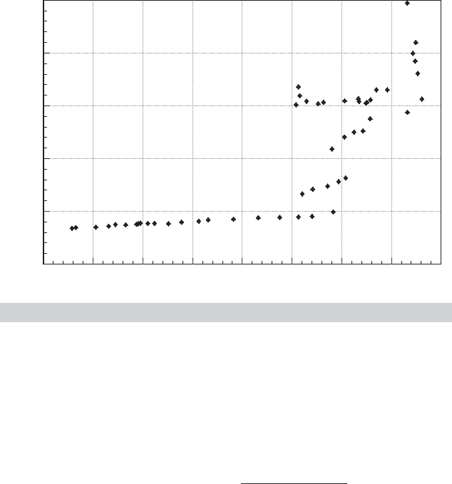
FIGURE 4.2

Per Capita Gasoline Consumption vs. Price, 1953–2004.

Each column of the K

× K

matrix P

1.2

is the column of slopes in the least squares

regression of the corresponding column of X

on the columns of X

Example 4.2 Omitted Variable

If a demand equation is estimated without the relevant income variable, then (4-10) shows

how the estimated price elasticity will be biased. The gasoline market data we have examined

in Example 2.3 provides a striking example. Letting b be the estimator, we obtain

E[b|price, income] = β +

Cov[price, income]

Var[price]

where γ is the income coefﬁcient. In aggregate data, it is unclear whether the missing co-

variance would be positive or negative. The sign of the bias in b would be the same as this

covariance, however, because Var[price] and γ would be positive for a normal good such as

gasoline. Figure 4.2 shows a simple plot of per capita gasoline consumption, G/Pop, against

the price index PG. The plot is considerably at odds with what one might expect. But a look

at the data in Appendix Table F2.2 shows clearly what is at work. Holding per capita income,

Income/Pop, and other prices constant, these data might well conform to expectations. In

these data, however, income is persistently growing, and the simple correlations between

G/Pop and Income/Pop and between PG and Income/Pop are 0.938 and 0.934, respectively,

which are quite large. To see if the expected relationship between price and consumption

shows up, we will have to purge our data of the intervening effect of Income/Pop.Todoso,

we rely on the Frisch–Waugh result in Theorem 3.2. In the simple regression of log of per

capita gasoline consumption on a constant and the log of the price index, the coefﬁcient is

0.29904, which, as expected, has the “wrong” sign. In the multiple regression of the log of

per capita gasoline consumption on a constant, the log of the price index and the log of per

capita income, the estimated price elasticity,

β,is−0.16949 and the estimated income elas-

ticity, ˆγ , is 0.96595. This conforms to expectations. The results are also broadly consistent

with the widely observed result that in the U.S. market at least in this period (1953–2004), the

main driver of changes in gasoline consumption was not changes in price, but the growth in

income (output).

PART I

✦

The Linear Regression Model

In this development, it is straightforward to deduce the directions of bias when there

is a single included variable and one omitted variable. It is important to note, however,

that if more than one variable is included, then the terms in the omitted variable formula

involve multiple regression coefﬁcients, which themselves have the signs of partial, not

simple, correlations. For example, in the demand equation of the previous example, if

the price of a closely related product had been included as well, then the simple corre-

lation between price and income would be insufﬁcient to determine the direction of the

bias in the price elasticity.What would be required is the sign of the correlation between

price and income net of the effect of the other price. This requirement might not be ob-

vious, and it would become even less so as more regressors were added to the equation.

4.3.3 INCLUSION OF IRRELEVANT VARIABLES

If the regression model is correctly given by

y = X

+ ε (4-12)

and we estimate it as if (4-8) were correct (i.e., we include some extra variables), then it

might seem that the same sorts of problems considered earlier would arise. In fact, this

case is not true. We can view the omission of a set of relevant variables as equivalent

to imposing an incorrect restriction on (4-8). In particular, omitting X

is equivalent

to incorrectly estimating (4-8) subject to the restriction β

=0. Incorrectly imposing a

restriction produces a biased estimator. Another way to view this error is to note that it

amounts to incorporating incorrect information in our estimation. Suppose, however,

that our error is simply a failure to use some information that is correct.

The inclusion of the irrelevant variables X

in the regression is equivalent to failing

to impose β

=0 on (4-8) in estimation. But (4-8) is not incorrect; it simply fails to

incorporate β

=0. Therefore, we do not need to prove formally that the least squares

estimator of β in (4-8) is unbiased even given the restriction; we have already proved it.

We can assert on the basis of all our earlier results that

E [b |X] =









. (4-13)

Then where is the problem? It would seem that one would generally want to “overﬁt”

the model. From a theoretical standpoint, the difﬁculty with this view is that the failure

to use correct information is always costly. In this instance, the cost will be reduced

precision of the estimates. As we will show in Section 4.7.1, the covariance matrix in

the short regression (omitting X

) is never larger than the covariance matrix for the

estimator obtained in the presence of the superﬂuous variables.

Consider a single-

variable comparison. If x

is highly correlated with x

, then incorrectly including x

the regression will greatly inﬂate the variance of the estimator of β

4.3.4 THE VARIANCE OF THE LEAST SQUARES ESTIMATOR

If the regressors can be treated as nonstochastic, as they would be in an experimental

situation in which the analyst chooses the values in X, then the sampling variance

There is no loss if X



= 0, which makes sense in terms of the information about X

contained in X

(here, none). This situation is not likely to occur in practice, however.