Greene W.H. Econometric Analysis

Подождите немного. Документ загружается.

CHAPTER 4

✦

The Least Squares Estimator

In a sample of 51 observations, one might argue that using the critical value for the limiting nor-

mal distribution might be a bit optimistic. If so, using the critical value for the t distribution with

51 −6 = 45 degrees of freedom would give a slightly wider interval. For example, for the the

income elasticity the interval would be 0.970523±2.014( 0.162386) = [0.643460, 1.297585].

We do note this is a practical adjustment. The statistic based on the asymptotic standard

error does not actually have a t distribution with 45 degrees of freedom.

4.5.3 CONFIDENCE INTERVAL FOR A LINEAR COMBINATION

OF COEFFICIENTS: THE OAXACA DECOMPOSITION

With normally distributed disturbances, the least squares coefﬁcient estimator, b,is

normally distributed with mean β and covariance matrix σ



−1

. In Example 4.8,

we showed how to use this result to form a conﬁdence interval for one of the elements

of β. By extending those results, we can show how to form a conﬁdence interval for a

linear function of the parameters. Oaxaca’s (1973) and Blinder’s (1973) decomposition

provides a frequently used application.

Let w denote a K × 1 vector of known constants. Then, the linear combination

c = w



b is normally distributed with mean γ = w



β and variance σ

= w



[σ



−1

]w,

which we estimate with s

= w



−1

]w. With these in hand, we can use the earlier

results to form a conﬁdence interval for γ :

Prob[c − t

(1−α/2),[n−k]

≤ γ ≤ c + t

(1−α/2),[n−k]

] = 1 −α. (4-43)

This general result can be used, for example, for the sum of the coefﬁcients or for a

difference.

Consider, then, Oaxaca’s (1973) application. In a study of labor supply, separate

wage regressions are ﬁt for samples of n

men and n

women. The underlying regression

models are

ln wage

m,i

= x



m,i

+ ε

m,i

, i = 1,...,n

and

ln wage

f, j

= x



f, j

+ ε

f, j

, j = 1,...,n

The regressor vectors include sociodemographic variables, such as age, and human cap-

ital variables, such as education and experience. We are interested in comparing these

two regressions, particularly to see if they suggest wage discrimination. Oaxaca sug-

gested a comparison of the regression functions. For any two vectors of characteristics,

E [ln wage

m,i

] − E [ln wage

f, j

f,i

] = x



m,i

− x



f, j

= x



m,i

− x



m,i

+ x



m,i

− x



f, j

= x



m,i

(β

− β

) + (x

m,i

− x

f, j

)



The second term in this decomposition is identiﬁed with differences in human capital

that would explain wage differences naturally, assuming that labor markets respond

to these differences in ways that we would expect. The ﬁrst term shows the differential

in log wages that is attributable to differences unexplainable by human capital; holding

these factors constant at x

makes the ﬁrst term attributable to other factors. Oaxaca

See Bourgignon et al. (2002) for an extensive application.

PART I

✦

The Linear Regression Model

suggested that this decomposition be computed at the means of the two regressor vec-

tors,

and x

, and the least squares coefﬁcient vectors, b

and b

. If the regressions

contain constant terms, then this process will be equivalent to analyzing

ln y

− ln y

We are interested in forming a conﬁdence interval for the ﬁrst term, which will

require two applications of our result. We will treat the two vectors of sample means as

known vectors. Assuming that we have two independent sets of observations, our two

estimators, b

and b

, are independent with means β

and β

and covariance matrices



)

−1

and σ



)

−1

. The covariance matrix of the difference is the sum of

these two matrices. We are forming a conﬁdence interval for



d where d = b

− b

The estimated covariance matrix is

Est. Var[d] = s



)

−1

+ s



)

−1

. (4-44)

Now, we can apply the result above. We can also form a conﬁdence interval for the

second term; just deﬁne w =

− x

and apply the earlier result to w



4.6 PREDICTION AND FORECASTING

After the estimation of the model parameters, a common use of regression modeling

is for prediction of the dependent variable. We make a distinction between “predic-

tion” and “forecasting” most easily based on the difference between cross section and

time-series modeling. Prediction (which would apply to either case) involves using the

regression model to compute ﬁtted (predicted) values of the dependent variable, ei-

ther within the sample or for observations outside the sample. The same set of results

will apply to cross sections, panels, and time series. We consider these methods ﬁrst.

Forecasting, while largely the same exercise, explicitly gives a role to “time” and often

involves lagged dependent variables and disturbances that are correlated with their

past values. This exercise usually involves predicting future outcomes. An important

difference between predicting and forecasting (as deﬁned here) is that for predicting,

we are usually examining a “scenario” of our own design. Thus, in the example below

in which we are predicting the prices of Monet paintings, we might be interested in

predicting the price of a hypothetical painting of a certain size and aspect ratio, or one

that actually exists in the sample. In the time-series context, we will often try to forecast

an event such as real investment next year, not based on a hypothetical economy but

based on our best estimate of what economic conditions will be next year. We will use

the term ex post prediction (or ex post forecast) for the cases in which the data used

in the regression equation to make the prediction are either observed or constructed

experimentally by the analyst. This would be the ﬁrst case considered here. An ex ante

forecast (in the time-series context) will be one that requires the analyst to forecast the

independent variables ﬁrst before it is possible to forecast the dependent variable. In

an exercise for this chapter, real investment is forecasted using a regression model that

contains real GDP and the consumer price index. In order to forecast real investment,

we must ﬁrst forecast real GDP and the price index. Ex ante forecasting is considered

brieﬂy here and again in Chapter 20.

CHAPTER 4

✦

The Least Squares Estimator

4.6.1 PREDICTION INTERVALS

Suppose that we wish to predict the value of y

associated with a regressor vector x

The actual value would be

= x

0

β + ε

It follows from the Gauss–Markov theorem that

ˆy

= x

0

b (4-45)

is the minimum variance linear unbiased estimator of E[y

] = x

0

β.Theprediction

error is

= ˆy

− y

= (b − β)



+ ε

The prediction variance of this estimator is

Var[e

|X, x

] = σ

+ Var[(b − β)



|X, x

] = σ

+ x

0





−1



. (4-46)

If the regression contains a constant term, then an equivalent expression is

Var[e

|X, x

] = σ

⎡

⎣

1 +

K−1



j=1

K−1



k=1



− ¯x



− ¯x







⎤

⎦

, (4-47)

where Z is the K − 1 columns of X not including the constant, Z



Z is the matrix of

sums of squares and products for the columns of X in deviations from their means [see

(3-21)] and the “jk” superscript indicates the jk element of the inverse of the matrix.

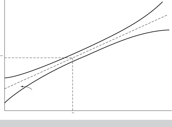
This result suggests that the width of a conﬁdence interval (i.e., a prediction interval)

depends on the distance of the elements of x

from the center of the data. Intuitively, this

idea makes sense; the farther the forecasted point is from the center of our experience,

the greater is the degree of uncertainty. Figure 4.5 shows the effect for the bivariate

case. Note that the prediction variance is composed of three parts. The second and third

become progressively smaller as we accumulate more data (i.e., as n increases). But,

the ﬁrst term, σ

is constant, which implies that no matter how much data we have, we

can never predict perfectly.

The prediction variance can be estimated by using s

in place of σ

. A conﬁdence

(prediction) interval for y

would then be formed using

prediction interval = ˆy

± t

(1−α/2),[n−K]





(4-48)

where t

(1−α/2),[n–K]

is the appropriate critical value for 100(1 − α) percent signiﬁcance

from the t table for n − K degrees of freedom and se(e

) is the square root of the

estimated prediction variance.

4.6.2 PREDICTING

WHEN THE REGRESSION MODEL

DESCRIBES LOG

It is common to use the regression model to describe a function of the dependent

variable, rather than the variable, itself. In Example 4.5 we model the sale prices of

Monet paintings using

ln Price = β

+ β

ln Area + β

AspectRatio + ε.

PART I

✦

The Linear Regression Model

a  b

冎

FIGURE 4.5

Prediction Intervals.

(Area is width times height of the painting and aspect ratio is the height divided by

the width.) The log form is convenient in that the coefﬁcient provides the elasticity of

the dependent variable with respect to the independent variable, that is, in this model,

= ∂ E[lnPrice|lnArea,AspectRatio]/∂lnArea. However, the equation in this form is

less interesting for prediction purposes than one that predicts the price, itself. The

natural approach for a predictor of the form

ln y

= x

0

would be to use

ˆy

= exp(x

0

b).

The problem is that E[y|x

] is not equal to exp(E[ln y|x

]). The appropriate conditional

mean function would be

E[y|x

] = E[exp(x

0

β + ε

)|x

]

= exp(x

0

β)E[exp(ε

)|x

The second term is not exp(E[ε

]) = 1 in general. The precise result if ε

normally distributed with mean zero and variance σ

is E[exp(ε

)|x

] = exp(σ

/2).

(See Section B.4.4.) The implication for normally distributed disturbances would be

that an appropriate predictor for the conditional mean would be

ˆy

= exp(x

0

b + s

/2)>exp(x

0

b), (4-49)

which would seem to imply that the na¨ıve predictor would systematically underpredict

y. However, this is not necessarily the appropriate interpretation of this result. The

inequality implies that the na¨ıve predictor will systematically underestimate the condi-

tional mean function, not necessarily the realizations of the variable itself. The pertinent

CHAPTER 4

✦

The Least Squares Estimator

question is whether the conditional mean function is the desired predictor for the ex-

ponent of the dependent variable in the log regression. The conditional median might

be more interesting, particularly for a ﬁnancial variable such as income, expenditure, or

the price of a painting. If the distribution of the variable in the log regression is symmet-

rically distributed (as they are when the disturbances are normally distributed), then

the exponent will be asymmetrically distributed with a long tail in the positive direction,

and the mean will exceed the median, possibly vastly so. In such cases, the median is

often a preferred estimator of the center of a distribution. For estimating the median,

rather then the mean, we would revert to the original na¨ıve predictor, ˆy

= exp(x

0

b).

Given the preceding, we consider estimating E[exp(y)|x

]. If we wish to avoid the

normality assumption, then it remains to determine what one should use for E[exp(ε

]. Duan (1983) suggested the consistent estimator (assuming that the expectation is a

constant, that is, that the regression is homoscedastic),

E[exp(ε

)|x

] = h



i=1

exp(e

), (4-50)

where e

is a least squares residual in the original log form regression. Then, Duan’s

smearing estimator for prediction of y

ˆy

= h

exp(x

0

b ).

4.6.3 PREDICTION INTERVAL FOR

WHEN THE REGRESSION

MODEL DESCRIBES LOG

We obtained a prediction interval in (4-48) for ln y|x

in the loglinear model lny =



β + ε,



ln ˆy

LOWER

, ln ˆy

UPPER





0

b − t

(1−α/2),[n−K]





, x

0

b + t

(1−α/2),[n−K]







For a given choice of α, say, 0.05, these values give the 0.025 and 0.975 quantiles of

the distribution of ln y|x

. If we wish speciﬁcally to estimate these quantiles of the

distribution of y|x

, not lny|x

, then we would use:



ˆy

LOWER

, ˆy

UPPER





exp



0

b −t

(1−α/2),[n−K]





, exp



0

b +t

(1−α/2),[n−K]





(4-51)

This follows from the result that if Prob[ln y ≤ ln L] = 1 − α/2, then Prob[ y ≤ L] =

1−α/2. The result is that the natural estimator is the right one for estimating the speciﬁc

quantiles of the distribution of the original variable. However, if the objective is to ﬁnd

an interval estimator for y|x

that is as narrow as possible, then this approach is not

optimal. If the distribution of y is asymmetric, as it would be for a loglinear model

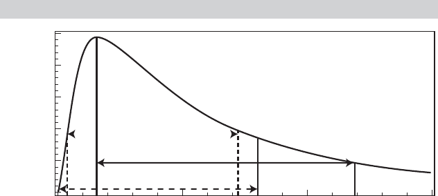
with normally distributed disturbances, then the na¨ıve interval estimator is longer than

necessary. Figure 4.6 shows why. We suppose that (L, U) in the ﬁgure is the prediction

interval formed by (4-51). Then, the probabilities to the left of L and to the right of U

each equal α/2. Consider alternatives L

= 0 and U

instead. As we have constructed

the ﬁgure, the area (probability) between L

and L equals the area between U

and U.

But, because the density is so much higher at L, the distance (0, U

), the dashed interval,

is visibly shorter than that between (L, U). The sum of the two tail probabilities is still

equal to α, so this provides a shorter prediction interval. We could improve on (4-51) by

PART I

✦

The Linear Regression Model

using, instead, (0, U

) where U

is simply exp[x

0

b + t

(1−α),[n−K]

se(e

)] (i.e., we put the

entire tail area to the right of the upper value). However, while this is an improvement,

it goes too far, as we now demonstrate.

Consider ﬁnding directly the shortest prediction interval. We treat this as an opti-

mization problem:

Minimize(L, U) : I = U − Lsubject to F(L) + [1 − F(U)] = α,

where F is the cdf of the random variable y (not lny). That is, we seek the shortest interval

for which the two tail probabilities sum to our desired α (usually 0.05). Formulate this

as a Lagrangean problem,

Minimize(L, U,λ) : I

∗

= U − L + λ[F(L) + (1 − F(U)) − α].

The solutions are found by equating the three partial derivatives to zero:

∂ I

∗

/∂ L =−1 + λ f (L) = 0,

∂ I

∗

/∂U = 1 −λ f (U) = 0,

∂ I

∗

/∂λ = F(L) + [1 − F(U)] − α = 0,

where f (L) = F



(L) and f (U) = F



(U) are the derivtives of the cdf, which are the

densities of the random variable at L and U, respectively. The third equation enforces

the restriction that the two tail areas sum to α but does not force them to be equal. By

adding the ﬁrst two equations, we ﬁnd that λ[ f(L) − f(U)] = 0, which, if λ is not zero,

means that the solution is obtained by locating (L

∗

, U

∗

) such that the tail areas sum to

α and the densities are equal. Looking again at Figure 4.6, we can see that the solution

we would seek is (L

∗

, U

∗

) where 0 < L

∗

< L and U

∗

< U

. This is the shortest interval,

and it is shorter than both [0, U

] and [L, U]

This derivation would apply for any distribution, symmetric or otherwise. For a

symmetric distribution, however, we would obviously return to the symmetric inter-

val in (4-51). It provides the correct solution for when the distribution is asymmetric.

FIGURE 4.6

Lognormal Distribution for Prices of Monet Paintings.

10 15

0.1250

Density

0.1000

0.0750

0.0500

.....................................

0.0250

0.0000

CHAPTER 4

✦

The Least Squares Estimator

In Bayesian analysis, the counterpart when we examine the distribution of a parameter

conditioned on the data, is the highest posterior density interval. (See Section 16.4.2.)

For practical application, this computation requires a speciﬁc assumption for the dis-

tribution of y|x

, such as lognormal. Typically, we would use the smearing estimator

speciﬁcally to avoid the distributional assumption. There also is no simple formula to

use to locate this interval, even for the lognormal distribution. A crude grid search

would probably be best, though each computation is very simple. What this derivation

does establish is that one can do substantially better than the na¨ıve interval estimator,

for example using [0, U

Example 4.10 Pricing Art

In Example 4.5, we suggested an intriguing feature of the market for Monet paintings, that

larger paintings sold at auction for more than than smaller ones. In this example, we will

examine that proposition empirically. Table F4.1 contains data on 430 auction prices for

Monet paintings, with data on the dimensions of the paintings and several other variables

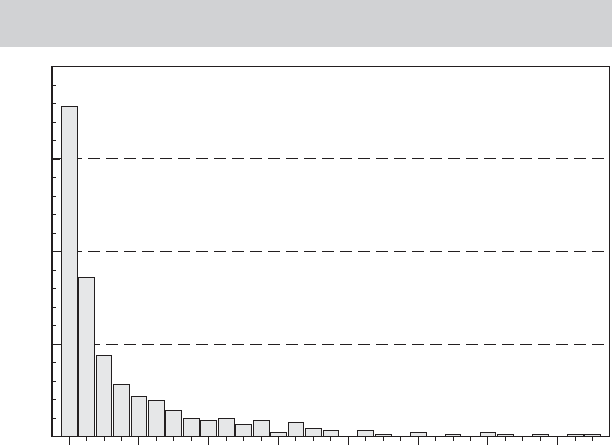
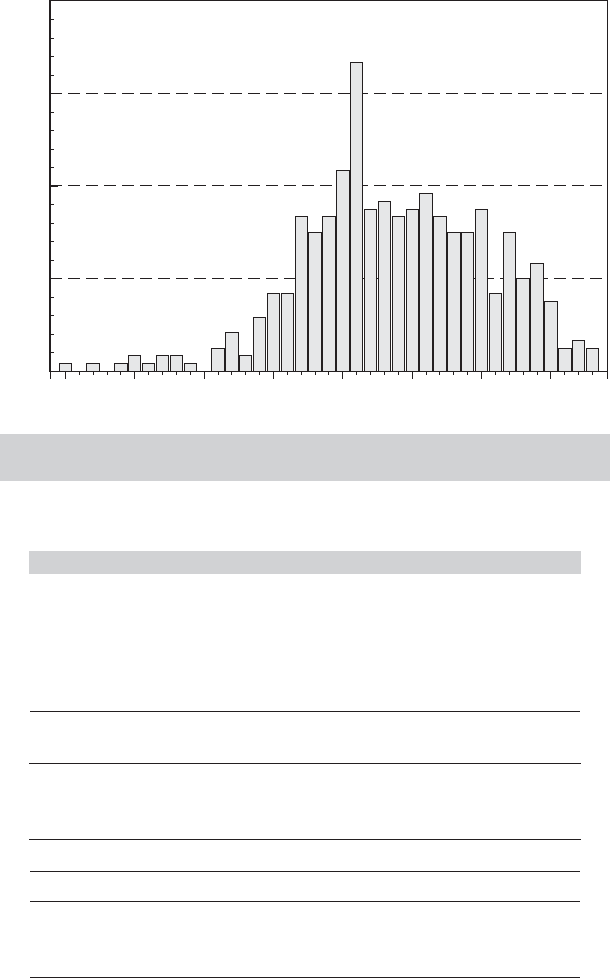
that we will examine in later examples. Figure 4.7 shows a histogram for the sample of sale

prices (in $million). Figure 4.8 shows a histogram for the logs of the prices.

Results of the linear regression of lnPrice on lnArea (height times width) and Aspect Ratio

(height divided by width) are given in Table 4.6.

We consider using the regression model to predict the price of one of the paintings, a 1903

painting of Charing Cross Bridge that sold for $3,522,500. The painting is 25.6” high and 31.9”

wide. (This is observation 60 in the sample.) The log area equals ln(25.6 ×31.9) = 6.705198

and the aspect ratio equals 25.6/31.9 = 0.802508. The prediction for the log of the price

would be

ln P|x

=−8.42653 + 1.33372(6.705198) − 0.16537(0.802508) = 0.383636.

FIGURE 4.7

Histogram for Sale Prices of 430 Monet Paintings

(

million).

0.010 3.664 7.318 10.972 14.626

Price

18.279 21.933 25.587

180

135

Frequency

PART I

✦

The Linear Regression Model

4.565 3.442 2.319 1.196 .073

Log P

1.050 2.172 3.295

Frequency

FIGURE 4.8

Histogram of Logs of Auction Prices for Monet

Paintings.

TABLE 4.6

Estimated Equation for Log Price

Mean of log Price 0.33274

Sum of squared residuals 519.17235

Standard error of regression 1.10266

R-squared 0.33620

Adjusted R-squared 0.33309

Number of observations 430

Standard Mean

Variable Coefﬁcient Error t of X

Constant −8.42653 0.61183 −13.77 1.00000

LogArea 1.33372 0.09072 14.70 6.68007

AspectRatio −0.16537 0.12753 −1.30 0.90759

Estimated Asymptotic Covariance Matrix

Constant LogArea AspectRatio

Constant 0.37434 −0.05429 −0.00974

LogArea −0.05429 0.00823 −0.00075

AspectRatio −0.00974 −0.00075 0.01626

Note that the mean log price is 0.33274, so this painting is expected to sell for roughly

5 percent more than the average painting, based on its dimensions. The estimate of the

prediction variance is computed using (4-47); s

= 1.104027. The sample is large enough

to use the critical value from the standard normal table, 1.96, for a 95 percent conﬁdence

CHAPTER 4

✦

The Least Squares Estimator

interval. A prediction interval for the log of the price is therefore

0.383636 ± 1.96( 1.104027) = [−1.780258, 2.547529].

For predicting the price, the na¨ıve predictor would be exp(0.383636) = $1.476411M, which is

far under the actual sale price of $3.5225M. To compute the smearing estimator, we require

the mean of the exponents of the residuals, which is 1.813045. The revised point estimate

for the price would thus be 1.813045 ×1.47641 = $2.660844M—this is better, but still fairly

far off. This particular painting seems to have sold for relatively more than history (the data)

would have predicted.

To compute an interval estimate for the price, we begin with the na¨ıve prediction by simply

exponentiating the lower and upper values for the log price, which gives a prediction interval

for 95 percent conﬁdence of [$0.168595M, $12.77503M]. Using the method suggested in

Section 4.6.3, however, we are able to narrow this interval to [0.021261, 9.027543], a range

of $9M compared to the range based on the simple calculation of $12.5M. The interval divides

the 0.05 tail probability into 0.00063 on the left and 0.04937 on the right. The search algorithm

is outlined next.

Grid Search Algorithm for Optimal Prediction Interval [LO, UO]

= (1,log(25.6 × 31.9), 25.6/31.9)



;

ˆμ

= ex p(x

0

b), ˆσ



+ x

0



−1

;

Conﬁdence interval for logP|x

: [Lower, Upper] = [ˆμ

− 1.96 ˆσ

,ˆμ

+ 1.96 ˆσ

];

Na¨ıve conﬁdence interval for Price|x

:L1= exp(Lower) ; U1 = exp(Upper);

Initial value of L was .168595, LO = this value;

Grid search for optimal interval, decrement by  = .005 (chosen ad hoc);

Decrement LO and compute companion UO until densities match;

(*) LO = LO −  = new value of LO;

f(LO) =



LO ˆσ

√

2π



−1

exp



−



(lnLO − ˆμ

)/ ˆσ





;

F(LO) = ((ln(LO) – ˆμ

)/ ˆσ

) = left tail probability;

UO = exp( ˆσ



−1

[F(LO) + 0.95] + ˆμ

) = next value of UO;

f(UO) =



UOˆσ

√

2π



−1

exp



−



(lnUO− ˆμ

)/ ˆσ





;

1 − F(UO) = 1 − ((ln(UO) – ˆμ

)/ˆσ

) = right tail probability;

Compare f(LO) to f(UO). If not equal, return to (

∗

). If equal, exit.

4.6.4 FORECASTING

The preceding discussion assumes that x

is known with certainty, ex post, or has been

forecast perfectly, ex ante. If x

must, itself, be forecast (an ex ante forecast), then the

formula for the forecast variance in (4-46) would have to be modiﬁed to incorporate the

uncertainty in forecasting x

. This would be analogous to the term σ

in the prediction

variance that accounts for the implicit prediction of ε

. This will vastly complicate

the computation. Many authors view it as simply intractable. Beginning with Feldstein

(1971), derivation of ﬁrm analytical results for the correct forecast variance for this

case remain to be derived except for simple special cases. The one qualitative result

that seems certain is that (4-46) will understate the true variance. McCullough (1996)

presents an alternative approach to computing appropriate forecast standard errors

based on the method of bootstrapping. (See Chapter 15.)

PART I

✦

The Linear Regression Model

Various measures have been proposed for assessing the predictive accuracy of fore-

casting models.

Most of these measures are designed to evaluate ex post forecasts, that

is, forecasts for which the independent variables do not themselves have to be forecast.

Two measures that are based on the residuals from the forecasts are the root mean

squared error,

RMSE =



(

− ˆy

)

and the mean absolute error,

MAE =



− ˆy

where n

is the number of periods being forecasted. (Note that both of these, as well as

the following measures, below are backward looking in that they are computed using the

observed data on the independent variable.) These statistics have an obvious scaling

problem—multiplying values of the dependent variable by any scalar multiplies the

measure by that scalar as well. Several measures that are scale free are based on the

Theil U statistic:

U =

(1/n

)



(

− ˆy

)

(1/n

)



This measure is related to R

but is not bounded by zero and one. Large values indicate

a poor forecasting performance. An alternative is to compute the measure in terms of

the changes in y:



(1/n

)



(

y

−  ˆy

)

(1/n

)





y



where y

= y

– y

i−1

and  ˆy

= ˆy

− y

i−1

, or, in percentage changes, y

= (y

–

i−1

)/y

i−1

and  ˆy

= ( ˆy

− y

i−1

)/y

i−1

. These measures will reﬂect the model’s ability to

track turning points in the data.

4.7 DATA PROBLEMS

The analysis to this point has assumed that the data in hand, X and y, are well measured

and correspond to the assumptions of the model in Table 2.1 and to the variables

described by the underlying theory. At this point, we consider several ways that “real-

world” observed nonexperimental data fail to meet the assumptions. Failure of the

assumptions generally has implications for the performance of the estimators of the

See Theil (1961) and Fair (1984).

Theil (1961).