Greene W.H. Econometric Analysis

Подождите немного. Документ загружается.

CHAPTER 4

✦

The Least Squares Estimator

outcome is fairly benign. The sample does not contain as much information as we might

hope, but it does contain sufﬁcient information consistently to estimate β and to do

appropriate statistical inference based on the information we do have.

The more difﬁcult case occurs when the measurement error appears in the inde-

pendent variable(s). For simplicity, we retain the symbols I and I* for our observed and

theoretical variables. Consider a simple regression,

y = β

+ β

∗

+ ε,

where y is the perfectly measured dependent variable and the same measurement equa-

tion, I = I

∗

+w applies now to the independent variable. Inserting I into the equation

and rearranging a bit, we obtain

y = β

+ β

I + (ε − β

= β

+ β

I + v. (4-57)

It appears that we have obtained (4-56) once again. Unfortunately, this is not the case,

because Cov[I,v] = Cov[I

∗

+ w,ε − β

w] =−β

. Since the regressor in (4-57) is

correlated with the disturbance, least squares regression in this case is inconsistent.

There is a bit more that can be derived—this is pursued in Section 8.5, so we state it

here without proof. In this case,

plim b

= β

[σ

∗

/(σ

∗

+ σ

)]

where σ

∗

is the marginal variance of I*. The scale factor is less than one, so the least

squares estimator is biased toward zero. The larger is the measurement error variance,

the worse is the bias. (This is called least squares attenuation.) Now, suppose there are

additional variables in the model;

y = x



+ β

∗

+ ε.

In this instance, almost no useful theoretical results are forthcoming. The following fairly

general conclusions can be drawn—once again, proofs are deferred to Section 8.5:

1. The least squares estimator of β

is still biased toward zero.

2. All the elements of the estimator of β

are biased, in unknown directions, even

though the variables in x are not measured with error.

Solutions to the “measurement error problem” come in two forms. If there is outside

information on certain model parameters, then it is possible to deduce the scale factors

(using the method of moments) and undo the bias. For the obvious example, in (4-57),

if σ

were known, then it would be possible to deduce σ

∗

from Var[I] = σ

∗

+ σ

and

thereby compute the necessary scale factor to undo the bias. This sort of information is

generally not available. A second approach that has been used in many applications is

the technique of instrumental variables. This is developed in detail for this application

in Section 8.5.

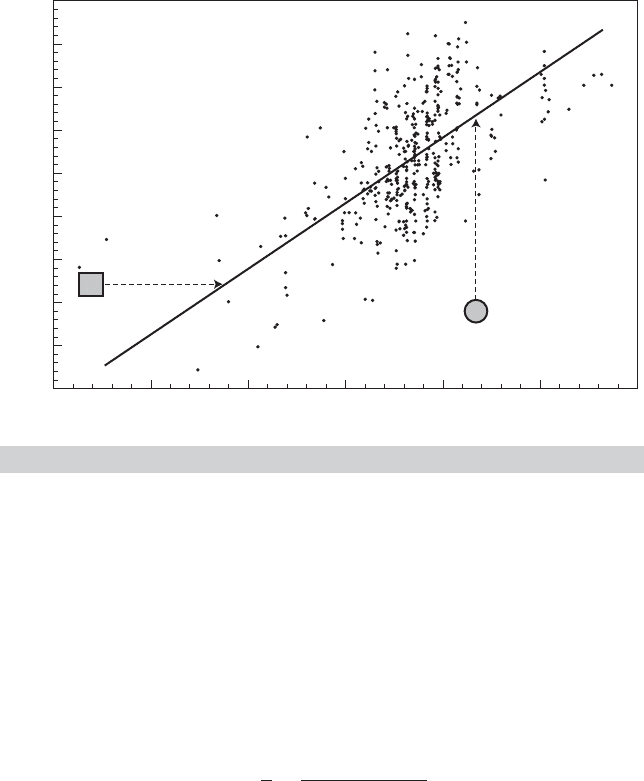
4.7.6 OUTLIERS AND INFLUENTIAL OBSERVATIONS

Figure 4.9 shows a scatter plot of the data on sale prices of Monet paintings that were

used in Example 4.10. Two points have been highlighted. The one marked “I” and noted

with the square overlay shows the smallest painting in the data set. The circle marked

100

PART I

✦

The Linear Regression Model

Log Area

4

3

2

1

5

4 5 6 7 8 93

Log Price

FIGURE 4.9

Log Price vs. Log Area for Monet Paintings.

“O” highlights a painting that fetched an unusually low price, at least in comparison

to what the regression would have predicted. (It was not the least costly painting in

the sample, but it was the one most poorly predicted by the regression.) Since least

squares is based on squared deviations, the estimator is likely to be strongly inﬂuenced

by extreme observations such as these, particularly if the sample is not very large.

An “inﬂuential observation” is one that is likely to have a substantial impact on the

least squares regression coefﬁcient(s). For a simple regression such as the one shown in

Figure 4.9, Belsley, Kuh, and Welsh (1980) deﬁned an inﬂuence measure, for observa-

tion i,

(

− ¯x

)



j=1

− ¯x

)

(4-58)

where ¯x

and the summation in the denominator of the fraction are computed without

this observation. (The measure derives from the difference between b and b

(i)

where

the latter is computed without the particular observation. We will return to this shortly.)

It is suggested that an observation should be noted as inﬂuential if h

>2/n. The de-

cision is whether to drop the observation or not. We should note, observations with

high “leverage” are arguably not “outliers” (which remains to be deﬁned), because the

analysis is conditional on x

. To underscore the point, referring to Figure 4.9, this obser-

vation would be marked even if it fell precisely on the regression line—the source of the

inﬂuence is the numerator of the second term in h

, which is unrelated to the distance of

the point from the line. In our example, the “inﬂuential observation” happens to be the

result of Monet’s decision to paint a small painting. The point is that in the absence of

an underlying theory that explains (and justiﬁes) the extreme values of x

, eliminating

CHAPTER 4

✦

The Least Squares Estimator

101

such observations is an algebraic exercise that has the effect of forcing the regression

line to be ﬁtted with the values of x

closest to the means.

The change in the linear regression coefﬁcient vector in a multiple regression when

an observation is added to the sample is

b − b

(i)

= b =

1 + x







(i)



−1





(i)



−1



− x



(i)



(4-59)

where b is computed with observation i in the sample, b

(i)

is computed without observa-

tion i and X

(i)

does not include observation i. (See Exercise 6 in Chapter 3.) It is difﬁcult

to single out any particular feature of the observation that would drive this change. The

inﬂuence measure,

= x







(i)



−1

K−1



j=1

K−1



k=1



i, j

− ¯x

n, j



i,k

− ¯x





(i)



, (4-60)

has been used to ﬂag inﬂuential observations. [See, once again, Belsley, Kuh, and Welsh

(1980) and Cook (1977).] In this instance, the selection criterion would be h

>2(K−1)/n.

Squared deviations of the elements of x

from the means of the variables appear in h

so it is also operating on the difference of x

from the center of the data. (See the

expression for the forecast variance in Section 4.6.1 for an application.)

In principle, an “outlier,” is an observation that appears to be outside the reach of

the model, perhaps because it arises from a different data generating process. Point “O”

in Figure 4.9 appears to be a candidate. Outliers could arise for several reasons. The

simplest explanation would be actual data errors. Assuming the data are not erroneous,

it then remains to deﬁne what constitutes an outlier. Unusual residuals are an obvi-

ous choice. But, since the distribution of the disturbances would anticipate a certain

small percentage of extreme observations in any event, simply singling out observa-

tions with large residuals is actually a dubious exercise. On the other hand, one might

suspect that the outlying observations are actually generated by a different population.

“Studentized” residuals are constructed with this in mind by computing the regression

coefﬁcients and the residual variance without observation i for each observation in the

sample and then standardizing the modiﬁed residuals. The ith studentized residual is

e(i) =

(1 − h

)



e − e

/(1 − h

)

n − 1 − K

(4-61)

where e is the residual vector for the full sample, based on b, including e

the residual

for observation i. In principle, this residual has a t distribution with n − 1 − K degrees

of freedom (or a standard normal distribution asymptotically). Observations with large

studentized residuals, that is, greater than 2.0, would be singled out as outliers.

There are several complications that arise with isolating outlying observations in

this fashion. First, there is no a priori assumption of which observations are from the

alternative population, if this is the view. From a theoretical point of view, this would

suggest a skepticism about the model speciﬁcation. If the sample contains a substan-

tial proportion of outliers, then the properties of the estimator based on the reduced

sample are difﬁcult to derive. In the next application, the suggested procedure deletes

102

PART I

✦

The Linear Regression Model

TABLE 4.9

Estimated Equations for Log Price

Number of observations 430 410

Mean of log Price 0.33274 0.36043

Sum of squared residuals 519.17235 383.17982

Standard error of regression 1.10266 0.97030

R-squared 0.33620 0.39170

Adjusted R-squared 0.33309 0.38871

Coefﬁcient Standard Error t

Variable n = 430 n = 410 n = 430 n = 410 n = 430 n = 410

Constant −8.42653 −8.67356 0.61183 0.57529 −13.77 −15.08

LogArea 1.33372 1.36982 0.09072 0.08472 14.70 16.17

AspectRatio −0.16537 −0.14383 0.12753 0.11412 −1.30 −1.26

4.7 percent of the sample (20 observations). Finally, it will usually occur that obser-

vations that were not outliers in the original sample will become “outliers” when the

original set of outliers is removed. It is unclear how one should proceed at this point.

(Using the Monet paintings data, the ﬁrst round of studentizing the residuals removes

20 observations. After 16 iterations, the sample size stabilizes at 316 of the original 430

observations, a reduction of 26.5 percent.) Table 4.9 shows the original results (from

Table 4.6) and the modiﬁed results with 20 outliers removed. Since 430 is a relatively

large sample, the modest change in the results is to be expected.

It is difﬁcult to draw a ﬁrm general conclusions from this exercise. It remains likely

that in very small samples, some caution and close scrutiny of the data are called for.

If it is suspected at the outset that a process prone to large observations is at work,

it may be useful to consider a different estimator altogether, such as least absolute

deviations, or even a different model speciﬁcation that accounts for this possibility. For

example, the idea that the sample may contain some observations that are generated

by a different process lies behind the latent class model that is discussed in Chapters 14

and 18.

4.8 SUMMARY AND CONCLUSIONS

This chapter has examined a set of properties of the least squares estimator that will

apply in all samples, including unbiasedness and efﬁciency among unbiased estimators.

The formal assumptions of the linear model are pivotal in the results of this chapter. All

of them are likely to be violated in more general settings than the one considered here.

For example, in most cases examined later in the book, the estimator has a possible

bias, but that bias diminishes with increasing sample sizes. For purposes of forming

conﬁdence intervals and testing hypotheses, the assumption of normality is narrow,

so it was necessary to extend the model to allow nonnormal disturbances. These and

other “large-sample” extensions of the linear model were considered in Section 4.4. The

crucial results developed here were the consistency of the estimator and a method of

obtaining an appropriate covariance matrix and large-sample distribution that provides

the basis for forming conﬁdence intervals and testing hypotheses. Statistical inference in

CHAPTER 4

✦

The Least Squares Estimator

103

the form of interval estimation for the model parameters and for values of the dependent

variable was considered in Sections 4.5 and 4.6. This development will continue in

Chapter 5 where we will consider hypothesis testing and model selection.

Finally, we considered some practical problems that arise when data are less than

perfect for the estimation and analysis of the regression model, including multicollinear-

ity, missing observations, measurement error, and outliers.

Key Terms and Concepts

•

Assumptions

•

Asymptotic covariance

matrix

•

Asymptotic distribution

•

Asymptotic efﬁciency

•

Asymptotic normality

•

Asymptotic properties

•

Attrition

•

Bootstrap

•

Condition number

•

Conﬁdence interval

•

Consistency

•

Consistent estimator

•

Data imputation

•

Efﬁcient scale

•

Estimator

•

Ex ante forecast

•

Ex post forecast

•

Finite sample properties

•

Gauss–Markov theorem

•

Grenander conditions

•

Highest posterior density

interval

•

Identiﬁcation

•

Ignorable case

•

Inclusion of superﬂuous

(irrelevant) variables

•

Indicator

•

Interval estimation

•

Least squares attenuation

•

Lindeberg–Feller Central

Limit Theorem

•

Linear estimator

•

Linear unbiased estimator

•

Maximum likelihood

estimator

•

Mean absolute error

•

Mean square convergence

•

Mean squared error

•

Measurement error

•

Method of moments

•

Minimum mean squared

error

•

Minimum variance linear

unbiased estimator

•

Missing at random

•

Missing completely at

random

•

Missing observations

•

Modiﬁed zero-order

regression

•

Monte Carlo study

•

Multicollinearity

•

Not missing at random

•

Oaxaca’s and Blinder’s

decomposition

•

Omission of relevant

variables

•

Optimal linear predictor

•

Orthogonal random

variables

•

Panel data

•

Pivotal statistic

•

Point estimation

•

Prediction error

•

Prediction interval

•

Prediction variance

•

Pretest estimator

•

Principal components

•

Probability limit

•

Root mean squared error

•

Sample selection

•

Sampling distribution

•

Sampling variance

•

Semiparametric

•

Smearing estimator

•

Speciﬁcation errors

•

Standard error

•

Standard error of the

regression

•

Stationary process

•

Statistical properties

•

Stochastic regressors

•

Theil U statistic

•

t ratio

•

Variance inﬂation factor

•

Zero-order method

Exercises

1. Suppose that you have two independent unbiased estimators of the same parameter

θ, say

and

, with different variances v

and v

. What linear combination

θ =

+ c

is the minimum variance unbiased estimator of θ?

2. Consider the simple regression y

= βx

+ε

where E [ε |x] = 0 and E [ε

|x] = σ

a. What is the minimum mean squared error linear estimator of β?[Hint: Let the

estimator be (

β =c



y). Choose c to minimize Var(

β)+(E(

β −β))

. The answer

is a function of the unknown parameters.]

104

PART I

✦

The Linear Regression Model

b. For the estimator in part a, show that ratio of the mean squared error of

β to

that of the ordinary least squares estimator b is

MSE [

β]

MSE [b]

(1 + τ

)

, where τ

[σ



Note that τ is the square of the population analog to the “t ratio” for testing

the hypothesis that β = 0, which is given in (5-11). How do you interpret the

behavior of this ratio as τ →∞?

3. Suppose that the classical regression model applies but that the true value of the

constant is zero. Compare the variance of the least squares slope estimator com-

puted without a constant term with that of the estimator computed with an unnec-

essary constant term.

4. Suppose that the regression model is y

= α + βx

+ ε

, where the disturbances

have f (ε

) = (1/λ) exp(−ε

/λ), ε

≥ 0. This model is rather peculiar in that all

the disturbances are assumed to be nonnegative. Note that the disturbances have

E [ε

] = λ and Var[ε

] = λ

. Show that the least squares slope is unbiased

but that the intercept is biased.

5. Prove that the least squares intercept estimator in the classical regression model is

the minimum variance linear unbiased estimator.

6. As a proﬁt-maximizing monopolist, you face the demand curve Q = α +β P +ε.In

the past, you have set the following prices and sold the accompanying quantities:

Q 337610151613915915121821

P 181617121515413116810777

Suppose that your marginal cost is 10. Based on the least squares regression, com-

pute a 95 percent conﬁdence interval for the expected value of the proﬁt-maximizing

output.

7. The following sample moments for x =[1, x

, x

] were computed from 100 ob-

servations produced using a random number generator:



X =

⎡

⎢

⎣

100 123 96 109

123 252 125 189

96 125 167 146

109 189 146 168

⎤

⎥

⎦

, X



y =

⎡

⎢

⎣

460

810

615

712

⎤

⎥

⎦

, y



y = 3924.

The true model underlying these data is y = x

+ x

+ ε.

a. Compute the simple correlations among the regressors.

b. Compute the ordinary least squares coefﬁcients in the regression of y on a con-

stant x

, x

, and x

c. Compute the ordinary least squares coefﬁcients in the regression of y on a con-

stant, x

and x

, on a constant, x

and x

, and on a constant, x

and x

d. Compute the variance inﬂation factor associated with each variable.

e. The regressors are obviously collinear. Which is the problem variable?

8. Consider the multiple regression of y on K variables X and an additional variable z.

Prove that under the assumptions A1 through A6 of the classical regression model,

the true variance of the least squares estimator of the slopes on X is larger when z

CHAPTER 4

✦

The Least Squares Estimator

105

is included in the regression than when it is not. Does the same hold for the sample

estimate of this covariance matrix? Why or why not? Assume that X and z are

nonstochastic and that the coefﬁcient on z is nonzero.

9. For the classical normal regression model y = Xβ + ε with no constant term and

K regressors, assuming that the true value of β is zero, what is the exact expected

value of F[K, n − K] = (R

/K)/[(1 − R

)/(n − K)]?

10. Prove that E [b



b] = β



β + σ



k=1

(1/λ

) where b is the ordinary least squares

estimator and λ

is a characteristic root of X



11. For the classical normal regression model y = Xβ + ε with no constant term and

K regressors, what is plim F[K, n − K] = plim

(1−R

)/(n−K)

, assuming that the true

value of β is zero?

12. Let e

be the ith residual in the ordinary least squares regression of y on X in the

classical regression model, and let ε

be the corresponding true disturbance. Prove

that plim(e

− ε

) = 0.

13. For the simple regression model y

= μ + ε

,ε

∼ N[0,σ

], prove that the sam-

ple mean is consistent and asymptotically normally distributed. Now consider the

alternative estimator ˆμ =



, w

(n(n+1)/2)



. Note that



= 1.

Prove that this is a consistent estimator of μ and obtain its asymptotic variance.

[Hint:



= n(n + 1)(2n + 1)/6.]

14. Consider a data set consisting of n observations, n

complete and n

incomplete,

for which the dependent variable, y

, is missing. Data on the independent variables,

, are complete for all n observations, X

and X

. We wish to use the data to

estimate the parameters of the linear regression model y = Xβ + ε. Consider the

following the imputation strategy: Step 1: Linearly regress y

on X

and compute

. Step 2: Use X

to predict the missing y

with X

. Then regress the full sample

of observations, (y

, X

), on the full sample of regressors, (X

, X

a. Show that the ﬁrst and second step least squares coefﬁcient vectors are identical.

b. Is the second step coefﬁcient estimator unbiased?

c. Show that the sum of squared residuals is the same at both steps.

d. Show that the second step estimator of σ

is biased downward.

15. In (4-13), we ﬁnd that when superﬂuous variables X

are added to the regression of

y on X

the least squares coefﬁcient estimator is an unbiased estimator of the true

parameter vector, β = (β



, 0



)



. Show that in this long regression, e



e/(n −K

−K

)

is also unbiased as estimator of σ

16. In Section 4.7.3, we consider regressing y on a set of principal components, rather

than the original data. For simplicity, assume that X does not contain a constant

term, and that the K variables are measured in deviations from the means and

are “standardized” by dividing by the respective standard deviations. We consider

regression of y on L principal components, Z = XC

, where L < K. Let d denote

the coefﬁcient vector. The regression model is y = Xβ + ε. In the discussion, it is

claimed that E[d] = C



β. Prove the claim.

17. Example 4.10 presents a regression model that is used to predict the auction prices

of Monet paintings. The most expensive painting in the sample sold for $33.0135M

(log = 17.3124). The height and width of this painting were 35” and 39.4”, respec-

tively. Use these data and the model to form prediction intervals for the log of the

price and then the price for this painting.

106

PART I

✦

The Linear Regression Model

Applications

1. Data on U.S. gasoline consumption for the years 1953 to 2004 are given in

Table F2.2. Note, the consumption data appear as total expenditure. To obtain

the per capita quantity variable, divide GASEXP by GASP times Pop. The other

variables do not need transformation.

a. Compute the multiple regression of per capita consumption of gasoline on per

capita income, the price of gasoline, all the other prices and a time trend. Report

all results. Do the signs of the estimates agree with your expectations?

b. Test the hypothesis that at least in regard to demand for gasoline, consumers do

not differentiate between changes in the prices of new and used cars.

c. Estimate the own price elasticity of demand, the income elasticity, and the cross-

price elasticity with respect to changes in the price of public transportation. Do

the computations at the 2004 point in the data.

d. Reestimate the regression in logarithms so that the coefﬁcients are direct esti-

mates of the elasticities. (Do not use the log of the time trend.) How do your

estimates compare with the results in the previous question? Which speciﬁcation

do you prefer?

e. Compute the simple correlations of the price variables. Would you conclude that

multicollinearity is a “problem” for the regression in part a or part d?

f. Notice that the price index for gasoline is normalized to 100 in 2000, whereas the

other price indices are anchored at 1983 (roughly). If you were to renormalize

the indices so that they were all 100.00 in 2004, then how would the results of the

regression in part a change? How would the results of the regression in part d

change?

g. This exercise is based on the model that you estimated in part d. We are inter-

ested in investigating the change in the gasoline market that occurred in 1973.

First, compute the average values of log of per capita gasoline consumption in

the years 1953–1973 and 1974–2004 and report the values and the difference. If

we divide the sample into these two groups of observations, then we can decom-

pose the change in the expected value of the log of consumption into a change

attributable to change in the regressors and a change attributable to a change in

the model coefﬁcients, as shown in Section 4.5.3. Using the Oaxaca–Blinder ap-

proach described there, compute the decomposition by partitioning the sample

and computing separate regressions. Using your results, compute a conﬁdence

interval for the part of the change that can be attributed to structural change in

the market, that is, change in the regression coefﬁcients.

2. Christensen and Greene (1976) estimated a generalized Cobb–Douglas cost func-

tion for electricity generation of the form

ln C = α + β ln Q + γ



(ln Q)



+ δ

ln P

+ δ

ln P

+ δ

ln P

+ ε.

, P

, and P

indicate unit prices of capital, labor, and fuel, respectively, Q is output

and C is total cost. To conform to the underlying theory of production, it is necessary

to impose the restriction that the cost function be homogeneous of degree one in

the three prices. This is done with the restriction δ

+δ

= 1, or δ

= 1 −δ

−δ

CHAPTER 4

✦

The Least Squares Estimator

107

Inserting this result in the cost function and rearranging produces the estimating

equation,

ln(C/P

) = α + β ln Q + γ



(ln Q)



+ δ

ln(P

) + δ

ln(P

) + ε.

The purpose of the generalization was to produce a U-shaped average total cost

curve. [See Example 6.6 for discussion of Nerlove’s (1963) predecessor to this study.]

We are interested in the efﬁcient scale, which is the output at which the cost curve

reaches its minimum. That is the point at which (∂ ln C/∂ ln Q)

|Q = Q

∗

= 1orQ

∗

exp[(1 − β)/γ ].

a. Data on 158 ﬁrms extracted from Christensen and Greene’s study are given in

Table F4.4. Using all 158 observations, compute the estimates of the parameters

in the cost function and the estimate of the asymptotic covariance matrix.

b. Note that the cost function does not provide a direct estimate of δ

. Compute

this estimate from your regression results, and estimate the asymptotic standard

error.

c. Compute an estimate of Q

∗

using your regression results and then form a con-

ﬁdence interval for the estimated efﬁcient scale.

d. Examine the raw data and determine where in the sample the efﬁcient scale lies.

That is, determine how many ﬁrms in the sample have reached this scale, and

whether, in your opinion, this scale is large in relation to the sizes of ﬁrms in

the sample. Christensen and Greene approached this question by computing the

proportion of total output in the sample that was produced by ﬁrms that had not

yet reached efﬁcient scale. (Note: There is some double counting in the data set—

more than 20 of the largest “ﬁrms” in the sample we are using for this exercise

are holding companies and power pools that are aggregates of other ﬁrms in

the sample. We will ignore that complication for the purpose of our numerical

exercise.)

HYPOTHESIS TESTS AND

MODEL SELECTION

5.1 INTRODUCTION

The linear regression model is used for three major purposes: estimation and prediction,

which were the subjects of the previous chapter, and hypothesis testing. In this chapter,

we examine some applications of hypothesis tests using the linear regression model. We

begin with the methodological and statistical theory. Some of this theory was developed

in Chapter 4 (including the idea of a pivotal statistic in Section 4.5.1) and in Appendix

C.7. In Section 5.2, we will extend the methodology to hypothesis testing based on the

regression model. After the theory is developed, Sections 5.3–5.7 will examine some

applications in regression modeling. This development will be concerned with the im-

plications of restrictions on the parameters of the model, such as whether a variable

is “relevant” (i.e., has a nonzero coefﬁcient) or whether the regression model itself is

supported by the data (i.e., whether the data seem consistent with the hypothesis that

all of the coefﬁcients are zero). We will primarily be concerned with linear restrictions

in this discussion. We will turn to nonlinear restrictions near the end of the development

in Section 5.7. Section 5.8 considers some broader types of hypotheses, such as choosing

between two competing models, such as whether a linear or a loglinear model is better

suited to the data. In each of the cases so far, the testing procedure attempts to resolve

a competition between two theories for the data; in Sections 5.2–5.7 between a narrow

model and a broader one and in Section 5.8, between two arguably equal models. Section

5.9 illustrates a particular speciﬁcation test, which is essentially a test of a proposition

such as “the model is correct” vs. “the model is inadequate.” This test pits the theory

of the model against “some other unstated theory.” Finally, Section 5.10 presents some

general principles and elements of a strategy of model testing and selection.

5.2 HYPOTHESIS TESTING METHODOLOGY

We begin the analysis with the regression model as a statement of a proposition,

y = Xβ + ε. (5-1)

To consider a speciﬁc application, Example 4.6 depicted the auction prices of paintings

ln Price = β

+ β

ln Size + β

AspectRatio + ε. (5-2)

Some questions might be raised about the “model” in (5-2), fundamentally, about the

variables. It seems natural that ﬁne art enthusiasts would be concerned about aspect ra-

tio, which is an element of the aesthetic quality of a painting.But, the idea that size should

108