Graziani F. (editor) Computational Methods in Transport

Подождите немного. Документ загружается.

512 C.J. Clouse

that passes through the container and strikes a detector on the far side of

the container. This is the classic source/detector problem of trying to get

adequate resolution at a detector that is far from the source; ray eﬀects can

be severe. We have been working on techniques that allow local adaptive

reﬁnement of the directional set of angles and expect to publish our results

in the near future. We also hope to extend the quadratic ﬁnite element in

angle [7] work to multi-dimensions to see if the substantial improvements in

convergence as a function of the number of angles holds for higher dimensions.

References

1. Clouse, C.: “Parallel 3D Neutronics on an AMR Grid”, Fifth Joint Russian

American Conference on Computational Mathematics, Sept. 22, 1997.

2. Clouse, C.: “Parallel Deterministic Neutron Transport with Adaptive Mesh

Reﬁnement”, 16th International Conference on Transport Theory, Georgia Tech

University, Atlanta, GA, May 14, 1999.

3. Baker R.: A Block Adaptive Mesh Reﬁnement Algorithm for the Neutral Par-

ticle Transport Equation. Nuc. Sci. & Eng., 141, 1–12 (2002)

4. Aussourd, C.: Styx: A Multidimensional AMR S

Scheme. Nuc. Sci. & Eng.,

143, 281–290 (2003)

5. Greenbaum, A. and J. Ferguson: A Petrov-Galerkin Finite Element Method for

Solving the Neutron Transport Equation. Journal of Comp. Phys., 64, 97–111

(1986)

6. Lewis, E. and W. Miller: Computational Methods of Neutron Transport, Wiley

and Sons, New York, 137–140 (1984)

7. Tolar, R. and J. Ferguson.: Quadratic Finite Element Method for 1D Deter-

ministic Transport. Trans. Am. Nucl. Soc., 90 (2004)

8. Berger, M. and P. Collela: Local Adaptive Mesh Reﬁnement for Shock Hydro-

dynamics. Journal of Comp. Phys., 82, 64–84 (1989)

9. Buck, R., E. Lent, T. Wilcox and S. Hadjimarkos: COG User’s Manual, ﬁfth

edition. Lawrence Livermore National Laboratory. (2002)

10. Compton, J. and C. Clouse: Domain Decomposition and Load Balancing in

the AMTRAN Neutron Transport Code, 15th Annual Conference on Domain

Decomposition Methods, Berlin, July (2003)

An Overview of Neutron Transport Problems

and Simulation Techniques

Edward W. Larsen

Department of Nuclear Engineering and Radiological Sciences, University of

Michigan, Ann Arbor, MI 48103-2109

edlarsen@umich.edu

1 Introduction

We brieﬂy summarize (i) the general characteristics of neutron (and photon)

transport processes relevant to nuclear reactor problems, (ii) the nature of

calculation techniques for these problems, and (iii) current areas of research

aimed at improving the accuracy and eﬃciency of these techniques.

2 Physical and Mathematical Basics

The problem of simulating the interaction of neutrons and photons with

matter has been an important calculational problem since the beginning of

“the nuclear era” – circa 1950. In large part, this is because nuclear reactors

now generate a substantial fraction of the electricity used by humankind.

In this brief review, we discuss (i) the physical and mathematical aspects

of neutron transport processes relevant to nuclear reactor problems, and (ii)

the main computational techniques that have been developed to solve these

problems. A very large literature on this subject has been published ([1–25]

are a few main sources), and we can do little but scratch the surface here.

Nonetheless, we hope to provide a useful overview of this interesting and

challenging ﬁeld.

In typical neutron transport problems, a physical system V and a source

of neutrons are speciﬁed. The source can be internal (within the system), or

external (e.g. a beam of neutrons incident on the outer surface ∂V of the

system). Individual neutrons, after being born, stream through the system

with ﬁxed directions of ﬂight and energies until they interact with nuclei or

leak out of the system. An interaction with a nucleus results in one of three

distinct types of events: (i) a capture event, in which the neutron is captured

by the nucleus, (ii) a scattering event, in which the neutron exchanges some

of its kinetic energy with the nucleus and departs with a diﬀerent energy

and direction of ﬂight, and (iv) a ﬁssion event, in which the nucleus splits

into two daughter nuclei, and one or more high-energy ﬁssion neutrons and

514 E.W. Larsen

other radiation are emitted. Each neutron that is emitted in a scattering or

ﬁssion event is subject to the same possible physical interactions as the parent

neutron. The general neutron transport problem is: given the physical system

and the neutron sources, determine the neutron ﬂux at all points within the

system. For shielding problems, the neutron and photon ﬂuxes must both be

calculated. (Photons, which are a byproduct of inelastic scattering and ﬁssion

events, undergo a similar transport process as neutrons, except that photons

do not induce ﬁssion.)

For steady-state problems, the mathematical equations that describe the

neutron transport process consist of the linear Boltzmann equation for the

angular ﬂux:

Ω

·∇ψ(r,Ω,E)+Σ

(r,E)ψ(r,Ω,E)



∞



4π

(r,Ω



· Ω,E



→ E)ψ(r,Ω



)dΩ



χ(r

,E)

4π



∞



4π

νΣ

(r,E



)ψ(r,Ω



)dΩ



Q(r

,E)

4π

∈ V,Ω∈ 4π, 0 <E<∞ , (1a)

and a boundary condition that prescribes the ﬂux incident on the outer

boundary of the system:

ψ(r

,Ω,E)=ψ

(r,Ω,E) ,r∈ ∂V , Ω · n < 0 , 0 <E<∞ . (1b)

The independent variables in (1) are the 3-D spatial variable r

=(x, y, z),

the 2-D angular or direction-of-ﬂight variable Ω

(a unit vector), and energy E.

Thus, unless spatial symmetries exist that reduce the number of independent

variables, phase space is 6-dimensional. The to-be-determined angular ﬂux ψ

is deﬁned by:

ψ(r

,Ω,E)dV dΩdE = the number of neutrons located in dV about r,

traveling in a direction in dΩ about Ω

with an energy in dE about E.(2)

where v =

2E/m is the neutron speed. (Thus, ψ/v = N is the neutron

density.) The remaining terms in (1) are speciﬁed cross sections or sources.

Thus, Σ

(r,E)isthetotal cross section, deﬁned by:

(r,E)ds = probability that a neutron at r with energy E

will experience an interaction with a nucleus

while traveling a distance ds;(3)

(r,Ω



· Ω,E



→ E)isthediﬀerential scattering cross section, deﬁned by:

Neutron Transport Problems and Simulation Techniques 515

(r,Ω



· Ω,E



→ E)dsdΩdE = probability that a neutron at r ,

traveling with direction Ω



and energy E



, will scatter into

dΩ about Ω

and dE about E while traveling a distance ds; (4)

(r,E)istheﬁssion cross section, deﬁned by:

(r,E)ds = probability that a neutron at r with energy E

will initiate a ﬁssion event while traveling a distance ds;(5)

ν is the mean number of ﬁssion neutrons emitted in a ﬁssion event, χ(r

,E)

is the ﬁssion spectrum, deﬁned by:

χ(r

,E)dE = the probability that a ﬁssion neutron, emitted at r,

will have energy in dE about E;(6)

Q(r

,E)isanisotropic interior source:

Q(r

,E)dV dE = the rate at which neutrons are isotropically

emitted in dV about r

and dE about E;(7)

and ψ

(r,Ω,E) is the prescribed incident ﬂux, which for r ∈ ∂V , n =the

unit outer normal vector to ∂V at S, Ω

·n < 0, and dS an increment of area

on ∂V at r

, is deﬁned by:

|Ω

· n|ψ

(r,Ω,E)dS dΩdE = the rate at which neutrons,

traveling in dΩ about Ω

and dE about E,

ﬂow into V through dS.(8)

Equations (1) describe a steady-state neutron transport problem with

no photons. If photons were included, a second transport equation for the

photon angular ﬂux would be required; this equation would not contain the

ﬁssion term on the right side of (1a), but it would contain extra source terms,

depending linearly on the neutron ﬂux ψ, that describe the production of

photons due to neutron ﬁssion and inelastic scattering.

Equations (1) are linear because neutrons are assumed to interact only

with nuclei, not with each other. In a cm

of a typical reactor core, there

are roughly 10

nuclei, and perhaps 10

(plus or minus a few orders of

magnitude) neutrons. Therefore, neutron-neutron interactions, which would

be nonlinear, are suﬃciently rare that they can be neglected.

If time-dependent problems were to be considered, extra equations for

the neutron precursors – ﬁssion neutrons that are emitted by radioactive

decay several seconds after the initiating ﬁssion event took place – would

have to be formulated and coupled to the time-dependent version of (1a).

The study of time-dependent reactor problems forms the specialized ﬁeld of

reactor kinetics.

516 E.W. Larsen

In many reactor design and safety problems, the space- and time-dependent

temperature of the reactor, T (r

,t) must be considered as an extra unknown.

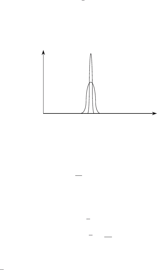
This is because cross sections are temperature-dependent; when tempera-

ture rises, Doppler-broadening causes narrow absorption resonances to widen,

leading to a small but signiﬁcant increase in the ability of the reactor to ab-

sorb neutrons. When T is included, an extra equation for T must be formu-

lated, and the cross sections in (1a) depend nonlinearly on T .

< T

(E,T)

Fig. 1. Doppler-Broadening of Capture Cross Section

In typical neutron transport problems, the total cross section and mean

free path satisfy

0.1cm

−1

<Σ

< 10.0cm

−1

, (9a)

0.1cm<λ=

= mean free path < 10.0cm, (9b)

with nominal values of Σ

≈ 1cm

−1

and λ ≈ 1 cm. Thus, neutron mean free

paths are generally orders of magnitude greater than electron or ion mean

free paths; this is because neutrons, which have no electrical charge, only

interact with atomic nuclei.

The mean scattering cosine

for neutron low-energy elastic scattering

is:

, (10)

where A is the mass number (number of neutrons plus protons) of the scatter-

ing nucleus. Thus, neutron scattering is generally much more isotropic than

typical electron scattering, which tends to be highly forward-peaked, with

≈ 1.

When fast neutrons scatter oﬀ nuclei, the neutrons typically exchange a

signiﬁcant fraction of their kinetic energy with the nuclei. For example, a

1.0 Mev neutron scattering in hydrogen (uranium) requires about 30 (2500)

scattering events to slow down to thermal (10

−2

ev) energies. (The lighter the

nucleus, the greater the energy exchange.) Electrons generally require orders

of magnitude more scattering events to undergo comparable energy losses.

Neutron Transport Problems and Simulation Techniques 517

Overall, the relatively large mean free path, large scattering angle, and

large energy loss of neutrons (compared with electrons) make (1) for neutrons

considerably more amenable to direct numerical simulation than the corre-

sponding equations for electrons. (Numerical methods for electron transport

problems nearly always use approximations necessitated by the extremely

small mean free path, scattering-angle, and energy-loss per collision.)

Core

Shield

4 m

Assembly

1 m

2 m

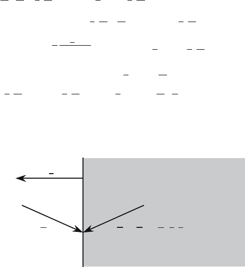
Fig. 2. Nuclear Reactor Schematic (Many Details Not Shown)

Figure 2 – a cartoon of a slice through a nuclear reactor – indicates a

central cylindrical core, consisting of a large array of long fuel assemblies

that contain the reactor fuel. (One fuel assembly is depicted.) Surrounding

the core is a reﬂector, and then a shield. (Only the shield is depicted.) Not

shown in the ﬁgure is the shielding on the top and bottom of the core. Also

not shown are the multitude of coolant channels passing through the core;

cold ﬂuid entering the core becomes hot as it passes through the core; when

it exits, the hot ﬂuid powers steam turbines, which then generate electricity.

In general, the reactor core contains a great deal of small-scale mechanical

structure; the reﬂector and shield, however, are basically homogeneous.

The fuel assemblies in reactor cores are generally arranged to maximize

eﬃciency and to ensure that the neutron ﬂux is relatively “ﬂat” across the

core. (However, due to the changes in cross sections from one material to

another, important space-dependent eﬀects deﬁnitely occur.) In the neutron

shield, surrounding the core, the neutron and photon density fall oﬀ – roughly

exponentially – by about 10 orders of magnitude from the interior wall of the

shield to the exterior wall. This fall-oﬀ (log scale) is depicted in Fig. 2.

518 E.W. Larsen

Equations (1) describe a ﬁxed-source problem for a physical system V .

Practical nuclear reactor neutron transport problems generally occur in three

categories:

1. Eigenvalue Calculations. Here the physical system V is the entire reactor,

the internal and boundary sources are set to zero, and the eigenvalue k

(the reactor criticality) is introduced in the denominator of the ﬁssion

term. Equations (1) become:

Ω

·∇ψ(r,Ω,E)+Σ

(r,E)ψ(r,Ω,E)



∞



4π

(r,Ω



· Ω,E



→ E)ψ(r,Ω



)dΩ



χ(r

,E)

4π



∞



4π

νΣ

(r,E



)ψ(r,Ω



)dΩ



∈ V,Ω∈ 4π, 0 <E<∞ , (11a)

ψ(r

,Ω,E)=0 ,r∈ ∂V , Ω · n < 0 , 0 <E<∞ . (11b)

The purpose of k is to adjust the amplitude of the ﬁssion process (which

adds new neutrons to the system), so that this process and the capture

and leakage processes (which delete neutrons from the system) exactly

balance, permitting a steady-state solution ψ to exist. The problem is

to determine a positive value of the eigenvalue k such that (11) have a

positive eigenfunction solution ψ.

If k>1, the ﬁssion process is suppressed to obtain a steady-state

solution, and the reactor is said to be supercritical.Ifk<1, the ﬁssion

process is enhanced to obtain a steady-state solution, and the reactor is

said to be subcritical.Ifk = 1, the the reactor is critical. A power reactor,

operating at steady state, is critical (k = 1). To increase the power out-

put of a critical reactor, control rods (which absorb neutrons) are slightly

withdrawn, causing k to become slightly greater than 1, thus causing the

neutron population within the reactor to slowly grow. Conversely, to de-

crease the power output of a critical reactor, control rods are slightly in-

serted, causing k to become slightly less than 1, thus causing the neutron

population within the reactor to slowly decline. Determining the critical-

ity k of a reactor is one of the fundamental problems in reactor design and

operation.

2. Assembly Calculations. Here the physical system V is a single reactor

assembly, all internal sources are set to zero, the eigenvalue k is introduced,

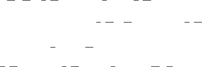
and reﬂecting (symmetry) boundary conditions are imposed on the outer

edges of the assembly to simulate an inﬁnite periodic system. If Ω

is the

specular reﬂection of the incident direction vector Ω

across the surface ∂V

of the assembly (see Fig. 3), then (1) become:

Neutron Transport Problems and Simulation Techniques 519

Ω ·∇ψ(r,Ω,E)+Σ

(r,E)ψ(r,Ω,E)



∞



4π

(r,Ω



· Ω,E



→ E)ψ(r,Ω



)dΩ



χ(r

,E)

4π



∞



4π

νΣ

(r,E



)ψ(r,Ω



)dΩ



∈ V,Ω∈ 4π, 0 <E<∞ , (12a)

ψ(r

,Ω,E)=ψ(r,Ω

,E) ,r∈ ∂V , Ω · n < 0 , 0 <E<∞ . (12b)

The problem is to determine a positive value of k such that (12) have a

positive (eigenfunction) solution ψ. [Note that this assembly-speciﬁc value

of k is generally not the criticality k of the reactor in (11).]

Ω

=Ω−

(Ω ⋅ n)nΩ

∂

Fig. 3. Reﬂecting (Symmetry) Boundary Condition)

The purpose of this calculation is to model the neutron ﬂux within

a single assembly. If all assemblies were identical, and if the the reactor

core were inﬁnite in extent, then (12) would correctly predict the criti-

cality k of the entire (inﬁnite) reactor, and the eigenfunction ψ, extended

periodically outside of the single assembly V , would correctly predict the

(periodic) eigenfunction of the inﬁnite reactor. However, reactor cores are

not inﬁnite, and fuel assemblies are not identical. Therefore, the neutron

ﬂux is not a periodic function of space. Nonetheless, for each assembly,

(12) are solved, and the results are processed to yield homogenized diﬀu-

sion coeﬃcients that, by means of a homogenized diﬀusion approximation,

predict (approximately) the variation of the amplitude of the neutron ﬂux

across the core. When this result is combined with the detailed eigen-

functions [obtained from (12) for each assembly], estimates of the neutron

ﬂux are obtained that are suﬃciently accurate for many applications. This

process, of solving many eigenvalue problems (one for each assembly) and

then “stitching” together a global solution, is often much more eﬃcient

than solving (11) for the entire reactor.

520 E.W. Larsen

3. Shielding Calculations. Here the physical system V is the reactor shield,

all internal sources (within the shield) are set to zero, the ﬁssion term is

set to zero (Σ

= 0 in a shield), and a prescribed incident neutron ﬂux ψ

representing the neutron ﬂux ﬂowing out of the core and into the shield,

is prescribed. Equations (1) become:

Ω

·∇ψ(r,Ω,E)+Σ

(r,E)ψ(r,Ω,E)



∞



4π

(r,Ω



· Ω,E



→ E)ψ(r,Ω



)dΩ



∈ V,Ω∈ 4π, 0 <E<∞ , (13a)

ψ(r

,Ω,E)=ψ

(r,Ω,E) ,r∈ ∂V , Ω · n < 0 , 0 <E<∞ . (13b)

The purpose of this calculation is to determine the extent to which the

shield absorbs the neutron and photon radiation from the reactor core,

and in particular, to calculate the radiation that successfully transmits

through the shield. In these problems, neutrons are usually suppressed

quickly; it is the high-energy photons, which are more deeply penetrat-

ing, that are problematic. To be complete, a second transport equation

and boundary conditions, closely resembling (13), should be added to de-

scribe the photon ﬂux. This second transport equation contains a source

term, depending linearly on the solution ψ of (13), which describes the

production of photons due to inelastic neutron scattering.

Unlike eigenvalue and assembly calculations, whose purpose is to deter-

mine the detailed neutron population in the reactor core, shielding cal-

culations are primarily performed to ensure that the reactors are safe –

that people can safely work outside the reactor, without an undue risk of

exposure to the radiation generated within the reactor.

For large commercial power reactors, practical neutron transport prob-

lems are rarely solved for the entire reactor system (full core plus shield); to

attempt this would generate a numerical problem that is much too large and

complex. Instead, much smaller “pieces” of the reactor are treated (e.g. a

single assembly, or the reactor shield) and the results combined in ways that

adequately approximate the neutron ﬂux across the entire system.

This completes our discussion of the basic mathematical and physical

description of neutron transport problems associated with the design and

operation of nuclear reactors. More detailed information on these topics can

be found in standard nuclear engineering texts: [1, 6–8], and [21].

Next, we discuss the two main computational approaches for simulat-

ing practical neutron transport problems: stochastic (i.e. Monte Carlo)and

deterministic techniques. Although these two approaches simulate the same

physical problem, they are (i) fundamentally diﬀerent in terms of their ap-

proach to the problem and their solution techniques, (ii) have been developed

by distinct computer code groups, (iii) exist only in separate computer codes,

Neutron Transport Problems and Simulation Techniques 521

and (iv) have complementary advantages and disadvantages. Because of this

complementarity, Monte Carlo and deterministic methods have each found

favor for certain types of problems. First, we discuss the basic concepts that

form the foundation of these two approaches.

3 Basics of Stochastic and Deterministic Methods

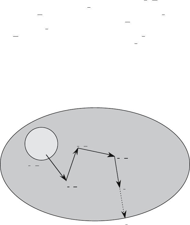
The physical process of neutron transport has at least one superﬁcially con-

tradictory aspect: the history of a single neutron is eﬀectively a sequence of

random events, while the solution of (1) contain no randomness. For example

(see Fig. 4), a single neutron is born at a random point (r

,Ω

) in phase

space, it streams to a random point r

where (let us say) it scatters into direc-

tion and energy Ω

and E

; then it streams to a random point r

where (let

us again say) it scatters into direction and energy Ω

and E

;thenitstreams

to a random point r

where (let us again say) it scatters into direction and

energy Ω

and E

; ﬁnally, it streams to a random point r

where it might be

captured – or, instead – it could stream to the point r

where it leaks out of

the system. Each particle history requires several random “decisions:” what

is the distance between collisions? When a collision occurs, is the collision a

scattering event, a ﬁssion event, or a capture event? If the particle scatters,

what are its outgoing energy and direction? For each neutron, these ques-

tions are answered by the rules of probability dictated by nature (through

the numerical values of the cross sections), and except for exceedingly rare

cases, the answers are diﬀerent.

Source

,Ω

, E

)

,Ω

)

,Ω

)

,Ω

, E

)

birth

scatter

capture

leaks out

Fig. 4. A Neutron History