Graziani F. (editor) Computational Methods in Transport

Подождите немного. Документ загружается.

460 R. McClarren et al.

This ﬂux can be transformed to the standard form of the Riemann solver

community by adding and subtracting



· (u

) r

to (13)

F(0,t)=



· u



· u



· u

−



· u

. (14)

Now looking at each term



· u

−



· u



· [u

− u

] r

= −



· [u

− u

] r

= −



· [∆u] r

(15)

where ∆u = u

− u

. The other terms



· u



· u



· u



· u

= Ru

(16)

Combining these to get

F(0,t)=Ru

−



· ∆ur

. (17)

Similarly, if we add and subtract



· u

to (13) the result is

F(0,t)=Ru



· ∆ur

. (18)

Averaging (17) and (18) gives

F(0,t)=

R(u

+ u

) −



|λ

· ∆ur

. (19)

The solution to the Riemann problem – the ﬂux between two cells – is writ-

ten in (19) as a centered-diﬀerence scheme plus the minimum amount of

dissipation to stabilize the scheme. However, the form in (13) shows us the

real power of using this approach. In this expression it is easily seen that

information is propagated upwind only, i.e. u

only contributes for positive

eigenvalues and u

only for negative eigenvalues. We could immediately use

this result in (2) by relabelling the l subscripts i − 1andther subscripts i.

Implicit Riemann Solvers for the P

Equations 461

4 High Resolution Flux from Linear Reconstruction

The preceding method for calculating the ﬂux between two cells is only ﬁrst

order in space when used on a cell-averaged quantities in solving a diﬀerential

equation. To create a scheme with greater spatial resolution we would like

to perform an interpolation of cell averaged quantities to reconstruct a more

precise value of ψ at the interface. A simple linear interpolation on each side

of the cell to get ψ

i±1/2

would be the obvious choice. However, Godunov’s

Theorem [Lev1992] tells us that linear reconstruction would only be ﬁrst

order in space if we prevent artiﬁcial oscillations (as we would be wont to

do). Ergo, we will use a nonlinear slope calculation which prevents artiﬁcial

maxima and minima creation (i.e. spurious oscillations).

The method ﬁrst suggested by Van Leer [Lev1992] for ﬂuid dynamics

applications and championed by Brunner [Bru2000] for particle transport is

the harmonic mean limiter. In this approach the slope at either side of an

interface is calculated using linear interpolation

−

− u

i−1

∆x

(20)

i+1

− u

∆x

, (21)

where u

is an element in the vector u

. Then we compute the harmonic mean

of the neighboring slopes

−

+ m

−

+ |m

−

| + |m

−

(22)

If the sign of m

−

does not equal the sign of m

thenweneedtosetm

because cell i is an extremum and interpolation could create artiﬁcial extrema

at its interfaces. Fortunately, the second form of the harmonic mean in (22)

does this automatically and does not compel the use of conditional statements

to check if each cell is an extreme point. In the case when both m

and m

−

are of the same sign, then we set

i±1/2

= u

∆x

. (23)

Withal, this method of reconstructing u

i±1/2

ensures that u

i±1/2

is always

between u

i−1

and u

i+1

This method has two new wrinkles compared to the ﬁrst-order scheme. In

that low-resolution scheme the average value or u

was used as the value at the

interfaces u

i±1/2

. The high-resolution method interpolates a linear function

to reconstruct the value of u

i±1/2

. This reconstruction does not take place at

extreme points in the values of u

; at these cells the method is still ﬁrst-order.

The other dissimilar facet of the high-resolution method is its nonlinearity, a

diﬀerence that will become signiﬁcant when treating the time integration.

462 R. McClarren et al.

The slope reconstruction method can be substituted into (19)

F(0,t)=



−

∆x

+ u

i−1

∆x

i−1



−



|λ



−

∆x

− u

i−1

−

∆x

i−1



. (24)

5 Time Integration

Now we have two expressions for the F’s in (2), for both high-resolution and

ﬁrst-order spatial schemes. There remains the time derivative component of

(2) to handle. We will do this using implicit time integration methods in order

to not be conﬁned by the Courant-Friedrichs-Lewy limit (c∆t/∆x < 1). The

backward (or implicit) Euler method is a ﬁrst order method given by setting

∂ψ

∂t

≈

(t + ∆t) −ψ

(t)

∆t

≡

n+1

− ψ

∆t

, (25)

and presuming all other instances of time-dependent quantities to be known

at time t + ∆t or time-step n + 1. This turns (2) into

n+1

− ψ

∆t

∆x



n+1

i+1/2

− F

n+1

i+1/2



= −Sψψ

n+1

+ Q

n+1

, (26)

Isolating the quantities at n +1

n+1

c∆t

∆x



n+1

i+1/2

− F

n+1

i+1/2



+ c∆tS

n+1

− c∆tQ

n+1

= ψψ

, (27)

which we write as

f(ψ

n+1

)=ψψ

. (28)

The problem given by (28) is a linear system in the case of the ﬁrst-order

spatial scheme, and nonlinear in the high-resolution case. For the ﬁrst-order

method, solving (28) involves solving a linear system of (N +1)I equations.

The nonlinear system for the high-resolution scheme has the same number of

equations.

A second-order time integration method, BDF2, was implemented as well.

This method has

∂u

∂t

≈

n−1

− u

∆x

n+1

− u

∆x

, (29)

and the other terms of the equation evaluated at time n + 1. This method

requires that the solution from the two previous time-steps be stored, a re-

quirement that could be problematic for large problems.

Implicit Riemann Solvers for the P

Equations 463

6 Implementation

This method for solving the P

equations was implemented in a C

code

named Implicit Riemann Object-Oriented Solver for the Transport of En-

ergetic Radiation (Implicit ROOSTER). This code uses the Trilinos solver

library, freely available from Sandia National Laboratory. For the solution

of the linear systems that arise in the ﬁrst-order spatial scheme, a restarted

GMRES solver is utilized (available in the AztecOO package of Trilinos).

The slope reconstruction method, the nonlinear system of equations is

treated using an inexact Newton method. The Newton iterations are deﬁned

j+1

= J

− (f (x

) − x

) , (30)

where the subscripts denote the j

approximation to the solution of f(x)=

and J is the Jacobian of f. This Jacobian is computed using a ﬁnite

diﬀerence method – meaning that we need not specify it explicitly. Further-

more, we have noticed that an eﬀectual preconditioner is the matrix from

the ﬁrst-order linear system. This is a reasonable preconditioner because the

high-resolution method is basically the ﬁrst-order method with a small cor-

rection term. Without this preconditioner the computational cost of even

a small problem was signiﬁcant; with it the computation time is not much

worse than the time for the ﬁrst-order method.

7 Results

To test the method we look at a Green’s function problem involving an

isotropic pulse of particles being emitted from a plane source in a 1D in-

ﬁnite medium at time t = 0. The medium is purely scattering with Σ

and c = 1. There is an analytic transport solution to this problem due

to Ganapol [Gan1986]. An analytic P

solution also exists for this prob-

lem [Bru2000]. The P

solution is characterized by a delta function of uncol-

lided particles travelling at speed ±

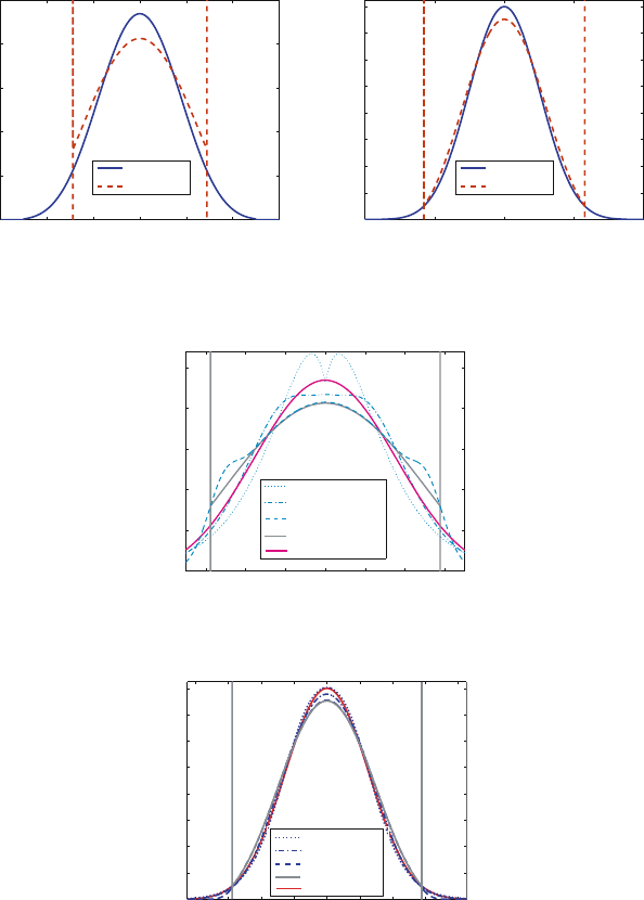
1/3. In Fig. 1 these exact solutions are

shown.

In Fig. 2 the numerical solutions 5 seconds after the pulse demonstrate a

smoothing of the spikes in the analytic P

solution. In this ﬁgure CFL =

∆x

∆t

and CFL > 1 would be unstable for an explicit time integration method.

Even time steps that allow particle to travel across ﬁfty spatial cells in one

time unit show excellent agreement with the analytic P

solution. It is clear

that the solutions are converging to the P

solution, as would be expected

for a method solving that P

equations in discretized form. Figure 3 shows

an interesting coincidence, namely that lower time ﬁdelity (i.e. longer time

steps) yields a solution nearer the transport solution. This is due to the fact

that implicit methods move particles at diﬀerent speeds than the continu-

ous time equations allow. In this problem, the P

speeds are not the correct

464 R. McClarren et al.

−6 −4 −2 0 2 4 6

Transport

Analytic P1

−10 −5 0 5 10

0.02

0.04

0.06

0.08

0.1

0.12

0.14

0.16

0.05

0.1

0.15

0.2

0.25

Transport

Analytic P1

Fig. 1. The analytic transport and P

solutions to the test problem at T =5and

T = 10 after the pulse

−3 −2 −1 3012

dt = 2.5 CFL = 1250

dt = 1, CFL = 500

Transport

Analytic P1

dt = 0.1, CFL = 50

0.05

0.1

0.15

0.2

0.25

Fig. 2. The high resolution P

solutions between x = −3.5 and 3.5atT =5

−8 −6 −4 −2 80246

Transport

dt = 2, CFL = 1000

dt = 1, CFL = 500

dt = 0 1, CFL= 50

Analytic P1

0.02

0.04

0.06

0.08

0.1

0.12

0.14

0.16

Fig. 3. The high resolution P

solutions at T = 10. The analytic P

solution and

the dt = 0.1 solution are coincident in the middle region

speeds for the transport solution. Consequently, by advecting particles at

the wrong P

speeds the numerical results happen to be closer to the trans-

port solution than the P

solution. However, more importantly the numerical

scheme converged in time captures the analytic P

solution. To test the time

Implicit Riemann Solvers for the P

Equations 465

−6 −4 −2 0 2 4 6

Transport

dt = 0 1, CFL = 200

dt = 0 5, CFL = 1000

Analytic P1

0.05

0.1

0.15

0.2

0.25

Fig. 4. The high resolution P

solutions at T = 10 with small spatial cells, dx =

0.0005 and large CFL numbers

discretization, the spatial cells were shrunk to dx= 5 × 10

−4

. In Fig. 4 the

time integration error should dominate and the results show that it is still

possible to get reasonable solutions with CFL numbers as high as 10

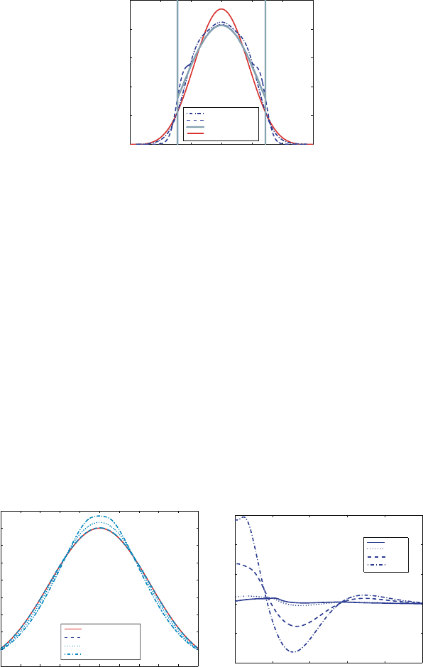
At T = 10 after the pulse of particles the numerical P

solution converged

in time is suﬃcient to capture the transport solution. This is demonstrated

in Fig. 5 where the φ

transport

− φ

≈10

−4

for dt= 10

−1

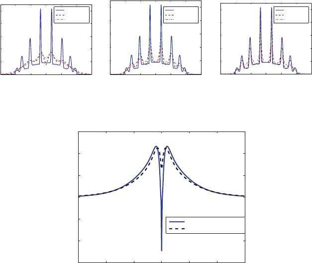
The high resolution and ﬁrst order spatial scheme was compared on a se-

ries of tests using the P

equations. The P

solutions have a series of “spikes”

representing the particles travelling at speeds characteristic of the P

equa-

tions – much like the delta functions of the P

equations. In the series of

plots in Fig. 6, the high resolution method captures these features more ac-

curately for coarse and ﬁne grids. This is advantageous insofar as the high

resolution method does not do worse than the ﬁrst-order scheme even on

these coarse grids. Finally, results from second-order time integration were

−5 −4 −3 −2 −1 0 1 2 3 4 5

0.02

0.04

0.06

0.08

0.1

0.12

0.14

0.16

0.18

Transport

dt = 0.1, CFL = 50

dt = 1, CFL = 500

dt = 2, CFL = 1000

−10−8−6−4−20

−0.01

−0.005

0.005

0.01

0.015

transport

−φ

dt = 0.1

dt = 1

dt = 2

dt = 02

Fig. 5. The P

solution and the diﬀerence between the transport ﬂux and computed

ﬂux at T =10

466 R. McClarren et al.

P7 at T=1, CFL = 0.25, N

= 50

1 0 5 0 5 1 510

P7 at T=1, CFL = 0.25, N

= 150

1 5 1 0 5 0 0 5 1 1 5

P7 atT=1, CFL = 0.25, N

= 300

HR, N

= 600

High Res

order

HR, N

= 600

High Res

order

HR, N

= 600

High Res

order

0 5

1 5

2 5

0 5

1 5

2 5

0 5

1 5

2 5

1 51 5 1 0 5 0 0 5 1 1 5

xxx

Fig. 6. Comparison of high resolution and ﬁrst-order solutions to the P

equations

with diﬀerent numbers of spatial grid points

−1.5 −1 0 1−0.5 0.5 1.5

BDF2, dt = 0.5

Backward Euler, dt = 0.5

−1.5

−1

−0.5

0.5

1.5

Fig. 7. The BDF2, high resolution P

solution at T = 1 has a negative scalar ﬂux

disheartening. Figure 7 shows the BDF2 solution compared with the back-

ward Euler solution. The negative ﬂux is not desirable. Also, it is worth

noting that in the previous ﬁgures the backward Euler method performed

well for large time steps. Moreover, other computations performed with the

BDF2 method demonstrated oscillations near extreme points in the solution.

8 Conclusion

We have presented an implicit Riemann solver for the P

equations. The

implicit Riemann solver gives good agreement with the transport solution

in regimes where the P

approximation is valid, even for large CFL num-

bers. The high resolution method is substantially better in capturing both

the sharp peaks in the solution and the smooth regions between. The test

problem was solved to impressive accuracy well beyond the CFL limit for the

approximation. The implicit integration “smooths” the delta functions

present in the analytic P

solution, which serendipitously allows large time

Implicit Riemann Solvers for the P

Equations 467

steps to agree with the transport solution better than smaller ones. Also, the

second-order time integration methods did not provide better answers for

time steps well beyond the CFL limit.

Currently, the authors are investigating diﬀusion limits for these methods

and how these Riemann solvers perform in the limit of optically thick cells.

Furthermore, the extension to higher dimensions and unstructured grids will

be pursued. The authors feel that the successes of implicit Riemann solvers

in one dimension portends successful results in two and three dimensions.

References

[BH2001a] Brunner, T., Holloway, J.P: One-Dimensional Riemann Solvers and

the Maximum Entropy Closure. Journal of Quantitative Spectroscopy

and Radiative Transfer, 69, 543–566 (2001)

[BH2001b] Brunner, T., Holloway, J.P: Two Dimensional Time Dependent Rie-

mann Solvers for Neutron Transport. Proceedings of the 2001 ANS

International Meeting on Mathematical Methods for Nuclear Applica-

tions, Salt Lake City, Utah, September 2001 (2001)

[Bru2000] Brunner, T.A.: Riemann Solvers for Time-Dependent Transport Based

on the Maximum Entropy and Spherical Harmonics Closures. PhD

Thesis, University of Michigan, Ann Arbor (2000)

[EPO2003] Eaton, M., Pain, C.C., de Oliveira, C.R.E., Goddard, A.: A High-Order

Riemann Method for the Boltzmann Transport Equation. Nuclear

Mathematical and Computational Sciences: A Century in Review; A

Century Anew, Gatlinburg, Tennesee, April 6–11 2003, (2003)

[Gan1986] Ganapol, B.D.: Solution of the One-Group Time-Dependent Neutron

Transport Equation in an Inﬁnite Medium by Polynomial Reconstruc-

tion. Nuclear Science and Engineering, 92, 272–279 (1986)

[Lev1992] Leveque, R.J.: Numerical Methods for Conservation Laws. Birkh¨auser

Verlag, (1992)

The Solution of the Time–Dependent S

Equations on Parallel Architectures

F. Douglas Swesty

State University of New York at Stony Brook

dswesty@mail.astro.sunysb.edu

1 Introduction

1.1 Motivation

The rapid growth of computing power, in the form of parallel architectures,

over the last decade has provided the unprecedented capability for computa-

tional scientists and engineers to carry out large scale simulations of radiation

transport and radiation-hydrodynamic phenomena. The development of mas-

sively parallel architectures on the scale of tens of thousands of processors

provides, in principle, the rate of ﬂoating point operations needed to carry

out multidimensional deterministic transport simulations involving multi-

ple physical timescales. However, this new technological advance presents a

tremendous challenge to the transport simulation developer in implementing

a method for the parallel solution of the time-dependent discrete-ordinates

Boltzmann equation on such platforms. Traditional iterative methods, such

as source iteration, that have been developed in many research communities

have undesirable features that present obstacles to eﬃcient parallelization. In

this paper we present an alternative approach, the full linear system solution

via Krylov subspace algorithms, that is more readily amenable to implemen-

tation on massively parallel architectures.

1.2 Requirements

The ultimate goal of this work is to ﬁnd an eﬃcient method to solve the

time-dependent discrete-ordinates transport equation on massively parallel

distributed memory. However, there are several desiderata for such a method:

• The solution should be highly scalable. The algorithm allow the eﬃcient

use of the largest possible number of processors in order to reduce the

wall clock time to solution for large long timescale problems that are

often associated with radiation heating or cooling of material. Another

way to state this criterion is that we desire a ﬁxed-size problem to scale

well to large numbers of processors even though the work per processor is

diminishing. We refer to such scaling as strong scaling. This is in contrast

to ﬁxed-work-per-processor scaling which is much easier to achieve.

470 F.D. Swesty

• The overall method should not be sensitive to the particulars of the

spatial, energy, or angular discretization schemes. A desirable solution

method would also be able to be employed with curvilinear coordinate

schemes as well as Cartesian coordinates. Ideally the method would also

be extendable to complex meshes such as block structured AMR meshes

or to unstructured meshes.

• The method should work well in the context of radiation-hydrodynamic

problems where the radiation is coupled to a ﬂuid. Ideally the method

would use the same spatial domain decomposition schemes that are em-

ployed for numerical hydrodynamic simulations.

• A solution method should be robust enough to handle scattering dom-

inated problems, problems with anisotropic scattering, and multigroup

problems with strong coupling between energy groups.

• The method should exploit the sparsity of the linear systems arising from

the implicitly discretized equations.

The aforementioned list of desiderata may seem overly constraining but

this list is compatible with the use of modern Krylov subspace algorithms

to solve the linear systems that arise from the implicit discretization of the

time-dependent Boltzmann equation.

2 A Brief Review of The Implicit Discrete Ordinates

Discretization Method

Before discussing approaches to implementing time-dependent Boltzmann

transport on parallel architectures we brieﬂy review the implicit discrete or-

dinates method for solving the monochromatic Boltzmann equation [MM99].

∂I

∂t

+ Ω ·∇I + κ

(ε)I −



dΩ





dε



I(Ω



,ε



)κ

(Ω



,ε



,Ω,ε)=

S(ε) . (1)

Throughout this paper we will utilize standard astrophysical nomenclature

and notation. In (1) I = I(x,Ω,ε,t) is the radiation intensity which is a

function of position x, direction Ω,energyε, and time t. For readers more

familiar with neutronics nomenclature can think of I as the ﬂux. The equation

involves material properties through the total opacity κ

(ε), the scattering

opacity κ

(Ω,ε, Ω



,ε



), and the emissivity S(ε). In (1) c denotes the speed of

light. Equation (1) describes the time evolution of particles traveling at the

speed of light such as photons or massless neutrinos, but it may be generalized

to describe massive particles such as neutrons by replacing c with the energy

dependent velocity v(ε).

This equation can be implicitly time-diﬀerenced as