Graziani F. (editor) Computational Methods in Transport

Подождите немного. Документ загружается.

502 C.J. Clouse

∂

∂t

Ω •

→

∇

+ σ



(2l +1)P



lg g



+ υσ

φ + q (4)

where

= angular ﬂux for energy group g and angle m,

= Legendre polynomial term l,

= total cross section for energy group g,

lg g



=thel

component of a Legendre polynomial expansion of the dif-

ferential scattering cross section from group g



to group g,

= the neutron velocity for group g.





(µ)Ψ



where m is the discrete angular index.

υσ

ϕ = represents the production of the scalar ﬂux into group g,andq

represents a possible, externally driven source term.

AMTRAN can solve (4) as either a ﬁxed source calculation (where q is

non-zero) or the usual k eigenvalue calculation, where k is a multiplier on

the ﬁssion source term, or α eigenvalue calculation where the time dependent

term is included in (4) and the time dependence is modeled as e

αt

. Equation

(4) is solved through standard source iteration and angular sweeps in which

the source terms on the right hand side of (4) are evaluated using the pre-

vious iterates values for the ﬂuxes. Then, with the value of S determined,

inversion of the sweeping term on the left hand side of (4) is accomplished

by sweeping through the mesh in the direction of neutron ﬂow; one sweep

for each unique combination of direction and energy group. This downwind

sweeping is complicated by block decomposition on a domain decomposed

mesh in which diﬀerent domains reside on diﬀerent processors. In order to

avoid idling processors, AMTRAN’s default domain decomposition is limited

to 8 domains (4 domains in 2D). By ensuring that each domain includes one

of the corners of the problem, all domains can immediately begin sweeping.

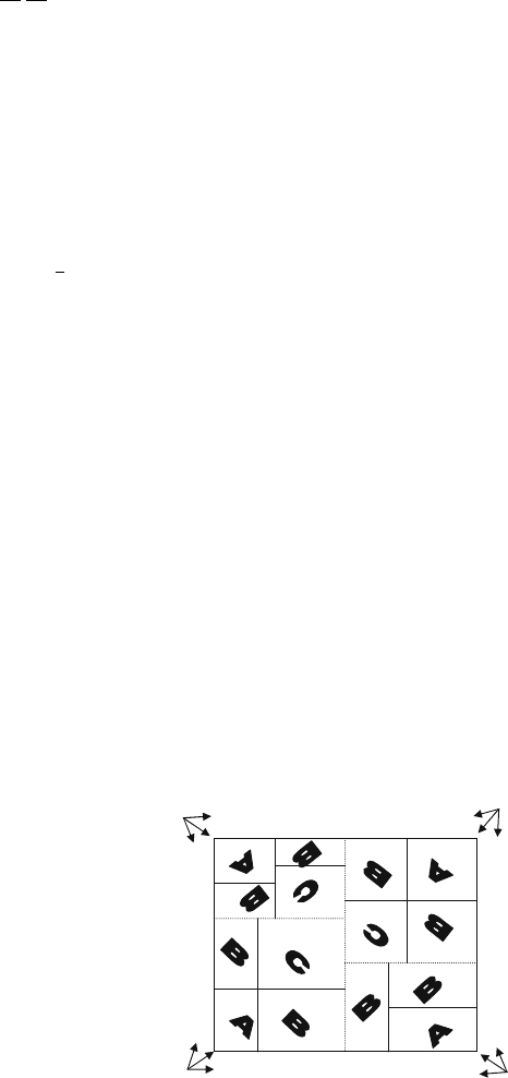
Figure 2 illustrates a simple 2D example assuming four spatial domains and

Fig. 2. Dashed lines indicate domain (and block) boundaries. Solid lines indicate

block boundaries

Parallel Deterministic Neutron Transport with AMR 503

12 angles. Each block designated “A” can be swept immediately by any one of

the three angles that originate from its corner. After any “A” block is swept,

its neighboring “B” blocks would have suﬃcient boundary information to

begin their sweep, followed by the “C” blocks, etc. A domain continues to

sweep blocks until no more blocks can be swept without receiving information

from neighboring domains, at which point it sends out all of its downwind

boundary information to the necessary neighboring domains and waits to re-

ceive upwind boundary information from any domains. AMTRAN assigns an

estimated weight to each zone in the generator mesh based on the mean free

path in that zone. This allows AMTRAN to estimate where to place domain

boundaries such that each domain has roughly equal weight and, therefore,

will have roughly equivalent zone counts after the AMR blocks are made. If

each domain has roughly equivalent zone counts, then each will ﬁnish their

sweeps at about the same time, pass information to and receive information

from neighboring domains, and continue sweeping with little or no idle time.

If there are reﬂecting boundaries in the problem, then the corners that lie on

reﬂecting boundaries will begin their sweeps with “old” boundary information

from the previous iteration. (Our deﬁnition of the term “iteration” is com-

parable to the standard textbook deﬁnition of an “outer iteration”, which

implies all angles have been swept through the entire mesh.) This causes

some degradation in the rate of convergence, but the fractional increase in

the number of iterations it takes to converge is usually substantially smaller

than the relative speedup achieved by simultaneously beginning sweeps from

all corners. For example, in 3D critical sphere calculations with one reﬂection

plane, the number of iterations required to achieve convergence is about 20%

more than the number of iterations required by ordering the sweeps such

that reﬂecting boundaries are not swept until incoming sweep information is

received, but the calculation will run roughly twice as slow by ordering the

sweeps since half the processors will be idle at any given time. Because eight

spatial domains (four in 2D) can be very limiting when attempting to scale up

to thousands of processors, recent work in AMTRAN has focused on eﬃcient

use of processors with more than eight spatial domains. Basically, the idea for

achieving high eﬃciency is through the use of domain overloading techniques.

We have created the construct of a domain master which represents a unique

collection of domains that may or may not be located contiguously in space.

Domains are assigned to domain masters in such a way as to keep the domain

master busy as much of the time as possible. Systematic algorithms have been

worked out that asymptotically approach 100% theoretical eﬃciency as the

number of domains per domain master is increased. The diﬀerence between

theoretical and actual eﬃciency is dependent on how well the code is able

to produce domains that are roughly equal in computational work, since the

algorithm assumes equal weight domains. Details of the algorithm have been

presented at an international conference [10], and will be outlined in a journal

article in the near future.

504 C.J. Clouse

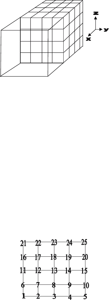
Fig. 3. A single zone from a coarse block that borders a ﬁner block along it’s x-face

2.3 Block Interfaces

As the sweeps proceed from block to block, three scenarios can occur at block

boundaries: (1) no change in zoning, (2) go from a coarser mesh to a ﬁner

mesh, (3) go from a ﬁner mesh to a coarser mesh. The ﬁrst scenario obvi-

ously requires no special treatment. The second scenario can be dealt with

in a straight forward fashion through bilinear interpolation of the coarse grid

ﬂuxes onto the ﬁne mesh. This is consistent with the linear ﬁnite element

representation of the ﬂuxes at the nodes. Unfortunately, the ﬁnite element

representation of the ﬂuxes at the nodes does not provide an obvious unique

solution to the third scenario, which is illustrated in Fig. 3. Over time, three

diﬀerent methods evolved in the code for treating scenario 3. The original

method, referred to as the pseudo-source method, is constrained by two cri-

teria: ﬂuxes of nodes at the same physical location on two diﬀerent mesh

should have the same value and ﬂux must be conserved across the interface.

To satisfy the ﬁrst criterion, we require that ﬂuxes at nodes 1, 5, 21 and 25

in Fig. 4 have the same value on the coarse and ﬁne blocks. If we integrate

(1) over a zone and focus on just the streaming term for the speciﬁc example

Fig. 4. Y-z interface of coarse to ﬁne zone. Fine zone nodes are numbered 1 to 25.

Coarse zone nodes are nodes 1, 5, 21 and 25

Parallel Deterministic Neutron Transport with AMR 505

shown in Figs. 3 and 4 with neutrons traveling in the +x direction, then the

ﬂux leaving the ﬁne zones overlapping the coarse zone can be written as,



i=1

+∆y



+∆z



dz dy (5a)

where, w

and w

are the y and z components of the linear ﬁnite element

weight functions at node 1, deﬁned as

=1−

−y)

dyf

for y

i−1

≥ y ≥ y

=1−

−z)

dzf

for z

i−1

≥ z ≥ z

=1−

(y−y

)

dyf

for y

i+1

≥ y ≥ y

=1−

(z−z

)

dzf

for z

i+1

≥ z ≥ z

=0 and,w

= 0 elsewhere,

and dyf = dzf =

∆y where ∆y = ∆z is the zone size on the coarse grid

and the coordinates of node 1 are given by (y

). Likewise, the ﬂux entering

the coarse zone can be expressed as



i=1,5,21,25

+∆y



+∆z



dz dy (5b)

where, w

and w

are the y and z components of the linear ﬁnite element

weight functions on the coarse zone at node 1, deﬁned as

=1−

− y)

∆y

for y

≥ y, w

=1−

− z)

∆z

for z

≥ z,

=1−

(y − y

)

∆y

for y ≥ y

=1−

(z − z

)

∆z

for z ≥ z

At the time boundary information is received, the diﬀerence between (5a)

and (5b) is calculated and stored as an additional zone centered source term

that is included in the solution of (4) and, thus, from the perspective of nodes

downwind from the boundary, the total ﬂux crossing from the ﬁne mesh to

the coarse mesh has been accounted for through the inclusion of an additional

source term, which we will refer to as the pseudo-source term. In a similar

fashion, the diﬀerence between the coarse and ﬁne mesh for the second term

on the left hand side of (4), the absorption term, is also accumulated into

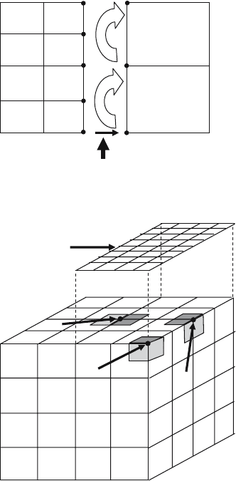
the pseudo-source term. The second method is referred to as the marching

method and is illustrated in Fig. 5. In this method, the value of the most

downwind node (node A in Fig. 5) is copied to the corresponding physical

node on the neighboring coarse grid (node F in Fig. 5). The value of node G

is then simply determined by ﬂux conservation across the interface between

nodes F and G. The value of node H is then determined by ﬂux conservation

across the interface between node G and H, etc.

506 C.J. Clouse

Direction of neutron flow

Fig. 5. Marching Method

Node C

Node B

Node A

Block I

Overlapping face of

Block II

Fig. 6. Area Weighting Method

The third method is referred to as the area weighting method and is

illustrated with a 3D example in Fig. 6. In our example, we have a coarse

block (block I) partially overlapped by a ﬁne block (block II) on the top face.

For neutrons incident on the upper right front corner, node C would not only

receive a ﬂux contribution from block II (indicated by the shaded area) but

also from two other blocks that overlap the two faces that are orthogonal to

the shaded face. The total contribution would be the area weighted sum of

the three incident faces. A corner node, like node C, can be shared by up to

8 blocks (in 3D), each of which may have a diﬀerent ﬂux value for that node.

Only in the case where all blocks sharing a node are at the same AMR level

are we guaranteed that all blocks see the same physical value. In the case of

node A, the lightly shaded area would contribute to the area weighted nodal

ﬂux, but if node A were located on the left edge of block I, then the lightly

Parallel Deterministic Neutron Transport with AMR 507

shaded area would either be located on a separate block or, in the case of block

I lying on the left edge of the problem, there would be no neighboring block.

In either case, the lightly shaded area would not contribute to node A’s value.

Likewise, if the direction of neutron ﬂow were from back to front, only the

shaded face, representing block II’s contribution, would contribute to node

C’s value. Thus, one can see that the area and number of faces contributing

to a nodal ﬂux value is dependent on the direction of neutron ﬂow. Method 1

is diﬃcult to implement in time-dependent problems and method 2 is prone

to instabilities. Thus, the default method used in AMTRAN is method 3.

2.4 Energy Group Parallelism

Distributed memory parallelism (i.e. the number of MPI processes spawned)

is equal to 8 (or 4 in 2D) x the number of energy groups per process. If

the number of processes is not evenly divisible by 8 (or 4 in 2D) then the

number of energy groups on a processor will vary by processor. In the case of

maximum parallelization, the user runs with one energy group per process.

Typically, in serial Sn codes, energy groups are swept sequentially from high-

est to lowest where the source term is updated after each energy group sweep

so that eﬀects from higher groups are immediately included in the lower

group sweeps, thus providing Gauss-Seidel like convergence on the iteration.

Therefore, in the case of no upscatter, the solution would converge after a

single iteration of all groups. In the case of maximum parallelization, which is

frequently the case in a typical AMTRAN calculation, all energy groups are

being solved simultaneously, using source terms calculated from the previous

iterate ﬂuxes and, therefore, the iterative technique is Jacobi-like rather than

Gauss-Seidel. One might expect a Jacobi solution to take more iterations to

converge than Gauss-Seidel however, in practice, what we observed for prob-

lems dominated by ﬁssion, and thus have large upscatter components, there

appears to be a break-even point at about 16 energy groups where, for prob-

lems with fewer than 16 energy groups, a Jacobi solution converges in fewer

iterations and with more than 16 energy groups, a Gauss-Seidel solution con-

verges in fewer iterations. The diﬀerence was not large, however, varying by

about +/−20% from 6 to 24 energy groups.

In AMTRAN, each process calculates it’s energy group(s) contribution

to the source term of each energy group in the problem. At this point, two

diﬀerent methods can be employed for communicating the results to the other

processes. The ﬁrst method is a tree-summing algorithm illustrated in Fig. 5

for a 4 group calculation with one energy group per process.

Many vendor implementations of MPI

−

Allreduce implement essentially

the same algorithm, however, we have seen MPI

−

Allreduce performance on

some machines to be substantially worse than our implementation of the

above algorithm and, therefore, we do not rely on the MPI

−

Allreduce call for

the summing of the sources since it can be a signiﬁcant fraction of the run

time of a calculation.

508 C.J. Clouse

Process 1

Ener

gy g

rou

Process 2

Ener

gy g

rou

Process 3

Ener

gy g

rou

Process 4

Ener

gy g

rou

Process 1

Process 3

Sum Sources

Process 1

Sum Sources

Broadcast results

Fig. 7. Tree-summing algorithm

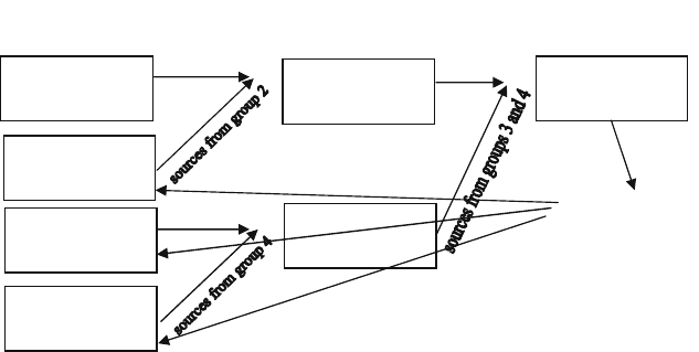
A second method takes advantage of the fact that a process only needs to

know what the source contributions are to it’s energy group(s). Thus, after

a process computes the contribution of its energy group(s) to all the oth-

ers, it sends individual messages to each process containing the contribution

to that process’ energy group(s). This is illustrated in Fig. 8. The method

illustrated in Fig. 7 requires 3(N-1) communications while that illustrated

in Fig. 8 requires N(N-1) communications, where N is the number of MPI

processes per domain. The messages in the second method, though, are much

smaller and less synchronized than those in the ﬁrst method and, as a result,

provide about a factor of 2 reduction in wall clock time for a 16 energy group

calculation on the IBM ASCI Paciﬁc Blue SP-2 machine at LLNL.

3 Numerical Results

As a simple numerical demonstration of the eﬀectiveness of spatial AMR, the

two-dimensional rod test case, as deﬁned in [4], will be used. This problem

consists of a cylindrical rod of

235

U surrounded by vacuum with a density

that decreases linearly from 66.71 g/cm

at the center plane to 20.09 g/cm

at the ends. All problems were run on LLNL’s Thunder machine, which is a

1024 node (four processors per node), 1.4 GHz Itanium machine. Aussourd

speciﬁes the ﬁnest level zoning to be 1 mm and gives results for up to 8 levels

of AMR, but states that eﬃciency gains beyond 3 levels are negligible and

tend to degrade accuracy. In fact, since the diﬀerence in density between the

peak value and the ends is only a little more than a factor of three and the

neutron mean free path varies linearly with the density, allowing more than

three levels violates AMTRAN’s default zoning criteria, since three levels

of reﬁnement already represents a factor of four diﬀerence in zone size for

Parallel Deterministic Neutron Transport with AMR 509

Process 1

Energy group 1

Process 2

Energy group 2

Process 3

Energy group 3

Process 4

Energy group 4

Process 1

Energy group 1

Process 2

Energy group 2

Process 3

Energy group 3

Process 4

Energy group 4

Fig. 8. Arrows for process 1 are labeled. Arrows for other processes would be

labeled in an analogous fashion

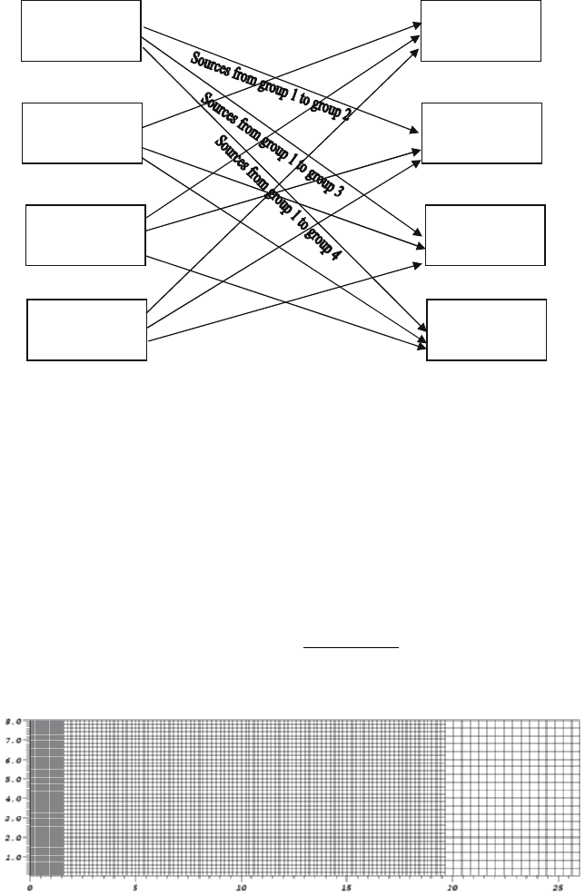
each direction. Figure 9 shows the zoning used by AMTRAN with three

levels of reﬁnement. Table 1 shows the results of several serial variations of

the calculations relative to a serial baseline calculation consisting of a single

block, uniformly zoned with 1 mm zoning. The k

eﬀ

of the baseline calculation

was 1.98480, which diﬀers slightly from [4]. This isn’t surprising since the

nuclear database and energy group resolution were not speciﬁed, so a direct

comparison could not be made. The relative error in Table 1 is deﬁned as:

Error = abs



1 −

1 − k

ef f

1 − k

baseline

ef f



(6)

Z (in cm)

R (in cm)

Fig. 9.

510 C.J. Clouse

Table 1.

Mesh Relative Relative compute Number of

Error time zones

Uniform, single block

(baseline calculation) 0 1 20800

Uniform, multi-block 0 0.95 20800

3 level AMR 2.0e-5 0.20 5200

Ref. 4 with 3 level AMR 4.1e-5 0.30 5760

and the relative compute time is just the ratio of the time for the calculation

relative to the baseline calculation:

Compute time =



time

baseline



(7)

The major diﬀerence between Aussourd’s [4] AMR method and our ap-

plication is our block based approach versus his tree based hierarchy. As he

points out, the advantage to a block based approach is it is more amenable

to spatial parallelism, but is less eﬃcient in reducing zone counts. A tree

based algorithm is better able to capture irregularly shaped gradients. Our

experience, however, has been that calculations generally run more eﬃciently

with liberal settings for the boxing eﬃciency; i.e. it is better to minimize the

number of blocks at the expense of running with more total zones. This as-

sumes, of course, that the diﬀerence in zone count is not too large; generally

no more than about 20%. If the diﬀerence is signiﬁcantly more that 20%, it

is probably worthwhile to increase the boxing eﬃciency.

Aussourd [4] reports roughly 40% overhead associated with the AMR logic

for this test problem. As can be seen from Table 1, we observe little, if any,

overhead. In fact, the multi-block logic, which is the major cost associated

with the AMR overhead of our block based approach, actually experiences a

5% reduction in run time for a uniform calculation relative to a single block

uniform calculation. This is most likely do to improved cache performance of

the multi-block approach since, if a block is small enough for all the unknowns

to ﬁt into cache, the sweeps can be performed without cache swapping. We

have seen this eﬀect in the past and, in fact, added an input variable which

allows users control over the maximum size of a block so calculations can

be tuned for diﬀerent architectures. This super-linear speedup is also seen in

the three level AMR calculation, which runs 5 times faster than the baseline

calculation despite the fact that the zone count is only reduced by a factor

of 4. It should be noted, though, that this particular test problem is ideally

suited for a block based AMR approach, since the gradients are planar.

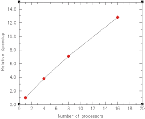
Figure 10 shows the relative speed improvement for the rod test problem

as a function of processor count. All points were run with the three level AMR

Parallel Deterministic Neutron Transport with AMR 511

Fig. 10. Relative speedup as a function of the number of processors for the rod

test problem (ﬁxed problem size)

version of the problem, giving a total of 5200 zones with 16 energy groups and

S10 quadrature. The 4, 8 and 16 processor runs used 4 spatial domains. The 8

processor run has two processors assigned per domain, and, therefore, would

be running with 8 energy groups per processor. The 16 processor run has 4

processors assigned per domain, thus giving 4 energy groups per processor.

Since there are two reﬂecting planes in this problem (the axis and z =0),

the domain decomposed problems take more iterations (∼20% increase) to

converge than does the serial calculation, so the timings have been normal-

ized to the iteration count of the serial calculation. As can be seen from the

plot, we achieve about a 12.8X speedup with 16 processors, giving an overall

parallel eﬃciency of 80%. The small problem size limits the degree of par-

allelism we can employ for this particular test case (the 16 processor run

completed 116 iterations in about 7 seconds). Two dimensional calculations

are commonly run that exceed 50,000 zones with 32 or more energy groups.

A large three dimensional calculation can have several million zones. These

kinds of calculations require hundreds to thousands of processors.

4 Future Work

Much of our recent eﬀort has been focused on the ability to reﬁne in direction.

Problems such as the neutron interrogation of a cargo container, mentioned

in Sect. 1, not only require spatial AMR because of the large problem dimen-

sions, but one is generally only interested in a narrow region of directional

phase space; basically the cone of angles, originating from a 14 MeV source,