Graziani F. (editor) Computational Methods in Transport

Подождите немного. Документ загружается.

336 R.M. Shagaliev et al.

∂

∂η

(B(η)N )+

∂

∂τ

(A(τ)N)+J(τ, η)ραN = J(τ,η)ρF

p(1,2)

− 6



−



p(3,4)

− 6N

(

p(1,2)

−

p(3,4)

)

−N

(

p(1,2)

p(3,4)

)+3

p(3,4)

η,p(1,4)

+ N

p(2,3)

+ SαN

= SF

p(4,1)

− 6



−



p(2,3)

− 6N

(

p(4,1)

−

p(2,3)

)

−N

(

p(4,1)

p(2,3)

)+3

p(1,2)

τ,p(1,2)

+ N

p(3,4)

+ SαN

= SF

¯χ

τ,12

− r

¯χ



−

τη



− r

+ A

)+3r

¯χ

η,41

−r

¯χ



−

τη



−

1 − µ

∆ϕ



sin ϕdϕ



ηϕ



+ J

τϕ



)

α(J

τη

+ J

τη

+ J

)

Some results of computational investigations for one test problem giving a

preliminary image of the main features of the scheme under consideration are

presented below. The results obtained using LMS scheme and the extended

template scheme used at present in SATURN-3 complex are compared.

Statement of the Test Problem

The linear time-independent particle transport problem (1)–(3) is considered

in axially symmetric region {0 ≤ R ≤ 1, 0 ≤ Z ≤ 2}. The source and the

equation coeﬃcients are taken as Q =1,α =1,β =1. The incoming ﬂow

equal to zero is speciﬁed for the boundaries parallel to R-axis (on the bases

of cylinder) and the boundary condition “mirror reﬂection” is speciﬁed for

the boundary parallel to Z-axis.

A series of computations was carried out using grids concentrating in an-

gular and spatial variables. An orthogonal uniform space grid was generated

for all the computations below.

1. Computation 1 (z1). The space grid has 10 rows and 10 columns. The an-

gular grid has 24 equal-area solid angles (the number of ranges in angular

variable µ is 6).

2. Computation 2 (z2). A space grid has 20 rows and 20 columns. The an-

gular grid has 84 equal-area solid angles (the number of ranges in angular

variable µ is 12).

3. Computation 3 (z3). A space grid has 40 rows and 40 columns. The angular

grid has 312 equal-area solid angles (the number of ranges in angular

variable µ is 12).

Finite-Diﬀerence Methods Implemented in SATURN Complex 337

2.5

3.5

4.5

0 0.2 0.4 0.6 0.8 1 1.2 1.4 1.6 1.8 2

cx.1 cx.1 cx.1 _ z1 _ z2 _ z3 lms_z1 lms_2 lms_z3

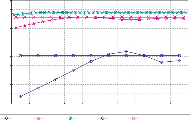
Fig. 8. Solution along the ﬁrst row

The distribution of particle density function n

(0)

obtained using the ex-

tended template scheme (scheme 1 in the following description) and LMS

scheme is considered as a result of computations. Figure 8 shows the solution

(density of particles n

(0)

) along the ﬁrst row corresponding to R = 1 that

has been obtained in 3 computations.

As one can see from the ﬁgure above, the solutions in the ﬁrst row ob-

tained using 2 various schemes coincide to a high precision (∼0.13% in com-

putation 1) and converge to the single solution.

Figure 9 shows the distribution of the particle density function along the

last row lying on Z-axis.

2.5

3.5

4.5

0 0.2 0.4 0.6 0.8 1 1.2 1.4 1.6 1.8 2

cx.1 _ z1 cx.1 _ z2 cx.1 _ z3 lms _ z1 lms _ z2 lms _ z3

Fig. 9. Solution along the last row

338 R.M. Shagaliev et al.

4.03

4.04

4.05

4.06

4.07

4.08

4.09

4.1

4.11

4.12

4.13

4.14

0 0.1 0.2 0.3 0.4 0.5 0.6 0.7 0.8 0.9 1

cx.1 _ z1 cx.1 _ z2 cx.1 _ z3 lms _ z1 lms _ z2 lms _ z3

Fig. 10. Solution along the central column

One can see here that solutions in the last row obtained using two various

schemes diﬀer from each other. For example, in computation 1, i.e. on the

coarsest grid, the discrepancy in solution is about 1.1%.

Figure 10 shows the proﬁle of solution along the central column. Note that

the solution along R-axis is one-dimensional (this follows from the problem

statement).

As one can see from the ﬁgure above, the use of LMS scheme does not lead

to the solution decrease along Z-axis and gives the solution constant to a high

precision. At the same time, there was some discrepancy in one-dimensional

behavior of solution in computations using the extended-template scheme

(∼1% in computation 1) typical of DSn–type schemes.

1.2 Adaptive Method of Reﬁned Grids in the Phase Space

The idea of the method under discussion is that in the phase region of the

problem solution some subregions are singled out, in which the original (ref-

erence) grid cells are reﬁned.

The major requirement imposed on the reﬁnement criteria and algorithms

is that of construction of grids adapted to the problem solution at a given

time in the phase space. This should eventually ensure a signiﬁcant saving

of the computational costs and, simultaneously, a needed accuracy of the

resultant numerical solution.

Finite-Diﬀerence Methods Implemented in SATURN Complex 339

The reﬁnement can be:

– in space variables;

– in angular variables;

– in energy variable.

In time-dependent problems the reference grid cell reﬁnement region is

redeﬁned at timesteps. In so doing special algorithms for selection of the

subregions and reﬁnement levels are involved.

The transport equation approximation on nonorthogonal spatial grids us-

ing the adaptive reﬁned grids entails the problem of preservation of the prin-

cipal properties of the scheme used for the numerical solution to the transport

equation on the reference grid, such as the transport equation approximation

within a single computational cell, conservatism of the scheme, the possibil-

ity to solve the grid transport equations with the point-to-point algorithm,

the possibility to use acceleration algorithms, and some others. An important

feature of the constructed adaptive method of reﬁned grids is that it ensures

the solution to the above problem.

Below are two examples of the 2D benchmark problem solution with the

adaptive method of reﬁned grids.

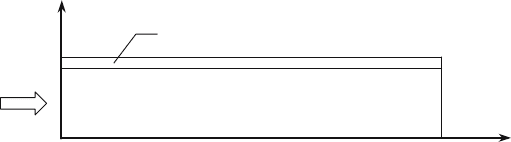
Benchmark problem. A rectangular region in 2D axisymmetric geome-

try is considered. The region is presented in Fig. 11. The computational

domain is composed of two physical regions: Physical region 1 is a dense

casing {0=Z =5;1=R =1.2}; Physical region 2 is a transparent region

{0=Z =5;0=R =1}.

Physical region 2

Physical region 1

1,2

Fig. 11. The system geometry in the 2D benchmark problem

The material density in the system is ρ = 1, the material energy as a

function of temperature is given with equation E =0.81 T . The computations

include photon absorption, with the photon absorption cross section being

given as χ

= A/T

. Diﬀerent values of the coeﬃcient A in the system give

optically dense region (Physical region 1) and optically transparent region

(Physical region 2). In Physical (optically dense) region 1 A = 50.89. In

Physical (optically transparent) region 2 A =0.1374. The scattering cross

section was taken zero (χ

= 0) in the computations. Initial temperature T

was assumed equal to 0.0001 at all the system points.

340 R.M. Shagaliev et al.

The following boundary conditions in radiation are given on the left end

of the rectangular domain {Z =0;1=R =1.2}: the “specular reﬂection”

condition is given on the boundary part referring to the dense casing and the

incoming isotropic radiation ﬂux corresponding to temperature T = 1 on the

part referring to the transparent region. On the upper boundary and on the

right end the incoming radiation ﬂux was given zero.

As a result, the solution to the equation of photon transport and radiation-

medium interaction is of a highly 2D nature in the problem under considera-

tion. The computations for the above problem employed the reference spatial

grid composed of 10 rows (5 in each of the physical regions) and 50 columns,

the angular grid included 16 spacings in angle µ and 6 spacings in ϕ,the

timestep was ∆t =0.00002. The computation on the spatial grid containing

40 × 200 cells was taken as the base computation and the resultant solution

is considered accurate.

Results of the computations using the adaptive technique. The spatial

grids, which the computations were performed on, are described below using

notation Nr (Pr) × Nz (Pz), where Nr is the number of rows, Nz is the number

of columns, Pr is the maximum adaptivity level in rows (MaxAdapt), Pz is

the maximum adaptivity level in columns. If no adaptivity is used in one of

the directions, the parameter in brackets is not speciﬁed.

The results of the 2D benchmark problem computation on the adaptive

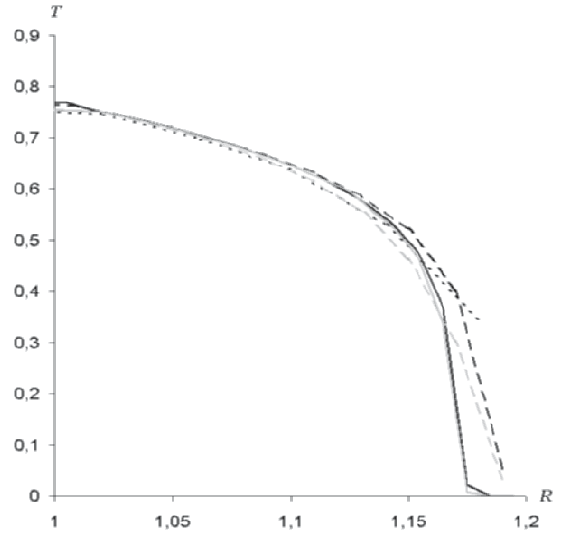
grids 10(4) × 50(4) and 10(8) × 50(8) are plotted in Fig. 12. For compari-

son that same ﬁgure presents the numerical solutions on some spatial grids

without the adaptivity.

As seen from the plots, the solution on grid 10(8) ×50(8) using the adap-

tive technique proves close to the result of the computation on grid 40 ×200

using the standard technique, with the adaptive computation requiring time

less by a factor of 2.8.

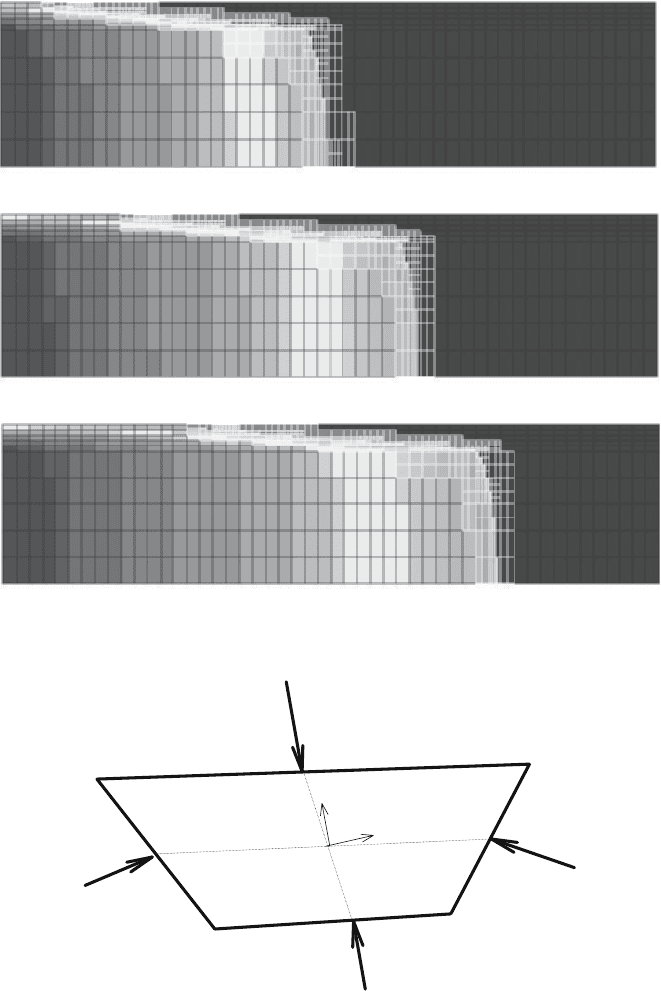
As an illustration demonstrating the results from the adaptive grid forma-

tion programs, Fig. 13 presents the radiation temperature ﬁeld distribution in

the system for three diﬀerent times. The black lines correspond to the refer-

ence spatial grid and the white lines to the adaptive cells. In the computation

the maximum adaptivity level is 2 (four adaptive cells in the reference grid)

along either direction. The adaptive partition of the spatial grid is seen to

proceed only at the wave front, with this being in diﬀerent ways in diﬀerent

spatial directions.

1.3 Algorithms for the Iterative Process Convergence

Acceleration in Complex SATURN

The numerical solution of many application problem classes requires methods

for acceleration of convergence of iterations in source (in the right-hand side

of the transport equation) to ensure the computation eﬃciency.

For the computations of linear time-independent problems of critical pa-

rameter calculation we have developed and are successfully using a ﬂow

Finite-Diﬀerence Methods Implemented in SATURN Complex 341

Fig. 12. Material temperature proﬁle along line Z = 2 at time 0.01 in the 2D

benchmark problem for diﬀerent reference grids: ——– solution on the base grid

40 × 200; – – – calculation 20 × 100; ······ – calculation 10 × 50; – – – calculation

10(4) × 50(4); —— calculation 10(8) × 50(8)

consistent acceleration method (FCA method). The brief formulation of the

method and some results of its numerical studies are presented below.

FCA Method (Flow Consistent Acceleration)

In the FCA method the following items are desired: functions of one-sided

ﬂow

⎧

⎪

⎨

⎪

⎩



(

Ω,¯n

)



Ω, ¯n



dΩ

−

= −



(

Ω,¯n

)



Ω, ¯n



dΩ

whose average grid values are introduced on the edges and medians of the grid

cells, function of total ﬂux W

= P

− P

−

given at the same points. Below

we introduce the average values on the scalar ﬂux function n

(0)



Ω

NdΩ

cell medians (Fig. 14).

342 R.M. Shagaliev et al.

t = 0.004

t = 0.006

t = 0.008

Fig. 13. Adaptive partition of spatial grid 10(8) × 50(8) at diﬀerent times

i, j

i+1, j

i+1, j+1

i, j+1

+1i

−

j+1/2

i+1/2

−

+1j

Fig. 14. The spatial grid cell

Finite-Diﬀerence Methods Implemented in SATURN Complex 343

Under these assumptions the diﬀerence equation system of the FSA

method is constructed using the integral moment equations, namely, the equa-

tions for zero and ﬁrst moments of function N of the solution to the

initial transport equation that include the compensating sources of the

simple iteration. To coordinate the solutions to the diﬀerence equations

S+1

+˜αN

S+1

=(βn

+ Q)

4π

used at the simple iteration phase and

at the simple iteration convergence acceleration phase, special grid functions

of the “compensating sources” are introduced to the right-hand sides of the

diﬀerence equations of the FCA method. The introduction of the functions

ensures convergence of the grid solution obtained by iterations with the FCA

method to the solution with the simple iteration method.



k∈(i,j,l)

(SL

− SL

k+1

)+(α − β) n

=(Q + F )

k+1/2



k+1

+ P

−

k+1



−



+ P

−



+ α · m · W

k+1/2

= FW

k+1/2

where k ∈ (i, j, l)

⎧

⎪

⎨

⎪

⎩



(

Ω,¯n

)



Ω, ¯n



dΩ

−

= −



(

Ω,¯n

)



Ω, ¯n



dΩ

= P

− P

−

, where k ∈ (i, j, l, i +1/2,j+1/2,l+1/2)

The grid equation set of the FCA method is closed with the relations of the

grid values given at diﬀerent points of the spatial cell:

k+1/2



δ · P

+(1− δ)P

k+1



+ Fδ

−

k+1/2



δ · P

−

k+1

+(1− δ)P

−



+ Fδ

−

, where k ∈ (i, j, l)

= AP



+ P

−



+ q

P k+

In the right-hand sides of the relations there are the grid functions of

the “compensating sources”. Like in the above equations, these sources are

introduced for the coordination of the grid solution obtained from the dif-

ference transport equations and the correction obtained from the diﬀerence

equations of the FCA method.

As the experience of using the FCA method suggests, in solution of com-

plex 2D application problems it reduces the time costs of the computations

by a factor up to 500. Below are examples of the computations for several

benchmark problems with the FCA method.

344 R.M. Shagaliev et al.

Region {0 <x<1.5, 0 <y<1.5, 0 <z<1.5}

2D 3D

αβN/A FCA N/A FCA

10. 9. 81 7 116 12

10. 9.9 331 7 300 13

10. 9.99 463 7 361 13

10. 10. 482 7 370 13

Results of the computations for reactor SNR-300

Method Number of Iterations

Kellog method 143

Direct method 141

Method of inverse iteration 112

Method of inverse iteration + FCA 20

Results of the computations for the RBMK reactor channel

Method Number of Iterations

Kellog method 229

Direct method 412

Source iteration method 555

Source iteration method + FCA 42

Source iteration method + FCA + Chebyshev method 24

Homogeneous sphere R =10

Number of Iterations

α = β Simple Iterations DSA Method FCA Method

1. 221 8 6

2. 597 8 6

4. 1627 9 6

8. 3927 8 6

12. 6003 12 6

16. 7658 24 9

Numerical Studies of the FCA Method for the Iterative Process

Convergence Acceleration

Particularly high requirements to the convergence and eﬃciency of the sim-

ple iteration convergence acceleration methods are imposed in solution to

nonlinear time-dependent multi-group X radiation transport problems.

Finite-Diﬀerence Methods Implemented in SATURN Complex 345

For this problem class, a so-called KM method was constructed by us as

early as the 1980s and improved in the recent years. The brief formulations

of the KM method and the improved KM method (KM3 method) and the

comparative results of the calculations with these methods for one time-

dependent benchmark problem are presented below.

The KM method is a two-step iterative method. At step 1 of the KM method

(predictor), the transport equation is solved with the method of simple iter-

ations (by source iterations).

n+1

−ε

∆t

+ L

n+γ

+α

n+γ

2π



j=1

(0)n+γ

n+γ

= γε

n+1

+(1− γ) ε

,i=1, 2,...,NI

At step 2 of the KM method (corrector), the correction equation system of

the following form is solved:

s+1

∆ε

n+1

∆t

+ L

s+1

∆ε

n+γ

+α

∆

s+1

n+γ

−



j=1

∆

s+1

n+γ

2π



j=1

∆ε

(0)n+γ

∆

s+1

−

s+1

∆ε

n+γ

= γ

s+1

∆ε

n+1

∆ε

(0)

−

(0)

,i=1, 2,...,NI

Mention some features of the group correction equations of KM-method

step 2:

1. The KM method is a conservative iterative method, with the two major

laws of conservation characteristic of the transport equation, i.e. the law

of conservation relative to the particle transport and that relative to the

medium-radiation energy exchange, being simultaneously satisﬁed at each

iterative process step.

2. The KM-method step 2 group equations are of the same form as the orig-

inal group transport equations, which allows the same diﬀerence methods

as those for the governing equations to be used for their grid approxima-

tion.

3. The cost-eﬃcient “point-to-point computation” method can be extended

to the numerical solution of the KM-method step 2 correction diﬀerence

group equation system.

KM3 Method

I step: predictor – like in the KM method