Graziani F. (editor) Computational Methods in Transport

Подождите немного. Документ загружается.

356 D.E. Shumaker and C.S. Woodward

we can write our discrete equations in terms of a discrete diﬀusion operator

given by

L(E

) ≡



1,1,1

), ···,L

)



, (4)

a local coupling operator given by

S(E

, E

) ≡ (S

1,1,1

, E

), ···,S

, E

))

, (5)

and the local reaction rate operator given by

R(E

,ρ

) ≡ (R

1,1,1

,ρ

), ···,R

,ρ

))

, (6)

where, as in [8]

i,j,k

) ≡



i+1/2,j,k

R,i+1,j,k

− E

R,i,j,k

∆x

i+1/2,j,k

− D

i−1/2,j,k

R,i,j,k

− E

R,i−1,j,k

∆x

i−1/2,j,k



/∆x

(7)



i,j+1/2,k

R,i,j+1,k

− E

R,i,j,k

∆y

i,j+1/2,k

− D

i,j−1/2,k

R,i,j,k

− E

R,i,j−1,k

∆y

i,j−1/2,k



/∆y



i,j,k+1/2

R,i,j,k+1

− E

R,i,j,k

∆z

i,j,k+1/2

− D

i,j,k−1/2

R,i,j,k

− E

R,i,j,k−1

∆z

i,j,k−1/2



/∆z

with the diﬀusion coeﬃcients evaluated on the face centers,

i+1/2,j,k

≡

3ρ

i+1/2,j,k

R,i+1/2,j,k

+ ∇E



i+1/2,j,k

R,i+1/2,j,k

i−1/2,j,k

≡

3ρ

i−1/2,j,k

R,i−1/2,j,k

+ ∇E



i−1/2,j,k

R,i−1/2,j,k

with y and z terms similarly deﬁned,

i,j,k

R,i,j,k

M,i,j,k

)=cρ

i,j,k

P,i,j,k



M,i,j,k

− E

R,i,j,k



, (8)

and

i,j,k

M,i,j,k

,ρ

F,i,j,k

)=σ

F,i,j,k



M,i,j,k



. (9)

Thus, our discrete scheme is to ﬁnd E

(t)andE

(t)suchthat,

= L(E

)+S(E

, E

), (10)

= −S(E

, E

)+e

R(E

,ρ

), (11)

dρ

= −R(E

,ρ

). (12)

For more details, see [7, 8].

Implicit Solution of Non-Equilibrium Radiation Diﬀusion 357

3.2 Time Integration and Solvers

We formulate (10)–(12) as an implicit system of ordinary diﬀerential equa-

tions (ODEs) and use an ODE time integrator to handle the implicit time

step selection. In particular, we employ the parallel ODE solver, CVODE [17],

developed at Lawrence Livermore National Laboratory and included in the

SUNDIALS package [18]. CVODE employs the ﬁxed leading coeﬃcient vari-

ant of the Backward Diﬀerentiation Formula (BDF) method [19, 20] and al-

lows for variation in the order of the time discretization as well as in the time

step size. Time step sizes are chosen to minimize the local truncation error

and thus give a solution that obeys a user-speciﬁed accuracy bound.

This time integration technique leads to a coupled, nonlinear system of

equations that must be solved at each time step. For example, solving the

ODE system

˙y = f(t, y), (13)

with the backward Euler method leads to the following nonlinear system

− y

n−1

∆t

= f(t

) (14)

that must be solved at each time step. For the solution of this system, we use

an inexact Newton–Krylov method with Jacobian-vector products approxi-

mated by ﬁnite diﬀerences. As the methods in CVODE are predictor-corrector

in nature, an explicit predictor (e.g., forward Euler in the case above) is used

for an initial guess in the nonlinear solve.

In the methods discussed above, we use the scaling technique incorpo-

rated into CVODE. Thus, we include an absolute tolerance (ATOL) for each

unknown and a relative tolerance (RTOL) which is applied to all unknowns.

These tolerances are then used to form a weight which is applied to each so-

lution component during the time step from t

n−1

to t

. This weight is given

= RT OL|y

n−1

| + AT OL

(15)

and is also used to weight a root mean square norm

y

WRMS



−1



)



1/2

(16)

which is applied to all error-like vectors within the solution process.

We use the GMRES Krylov iterative solver for solution of the linear Ja-

cobian system at each Newton iteration [21]. The tolerance for the Newton

iteration is taken to guarantee that iteration error introduced from the non-

linear solver is smaller than the local truncation error. For more details re-

garding the step size and order selection strategies in CVODE, as well as

acceptance of a step and nonlinear convergence, we refer the reader to the

review article [18].

358 D.E. Shumaker and C.S. Woodward

3.3 Preconditioning

Preconditioning is generally essential when using Krylov linear solvers. To

describe our preconditioning strategy, we begin by considering the content

and structure of the Jacobian matrix. In (13), set y =(E

, E

,ρ

)

and then form f using the right-hand sides of (10)–(12). The Jacobian ma-

trices used in the Newton method are of the general form F



(y)=(I − γJ),

where J = ∂f/∂y is the Jacobian of the nonlinear function f,andthepa-

rameter γ ≡ ∆tβ with ∆t the current time step value and β acoeﬃcient

depending on the order of the BDF method. Recalling the deﬁnitions of the

discrete divergence, coupling and reaction rate operators, the block form of

the Jacobian of f is

J =

⎛

⎝

∂L/∂E

+ ∂S/∂E

∂S/∂E

−∂S/∂E

+ e

∂R/∂E

∂R/∂ρ

0 −∂R/∂E

−∂R/∂ρ

⎞

⎠

⎛

⎝

A + GB 0

−G −B + e

0 −C −H

⎞

⎠

where A = ∂L/∂E

, G = ∂S/∂E

, B = ∂S/∂E

, C = ∂R/∂E

,and

H = ∂R/∂ρ

. We note that G, B, C and H are diagonal matrices. In all

of our preconditioning strategies, we neglect the nonlinearity in the diﬀusion

term and use the approximation [7, 8]

A = ∂L(

)/∂E

≈

) ≡

where ∂L(

)/∂E

is the Jacobian of L evaluated at a radiation energy,

The size of the neglected term is related to the derivatives of the Rosseland

opacity and the ﬂux-limiter. Our motivation for neglecting this term arises

from the fact that −

A is symmetric and positive deﬁnite, whereas −A is not,

and we thus can use multigrid methods for solution of diﬀusion terms within

the preconditioner.

Our preconditioning strategy is to factor the matrix, M ≡ I − γ

J,as

⎛

⎝

PQ0

UTV

0 YZ

⎞

⎠

≡

⎛

⎝

I − γ(

A + G) −γB 0

γG I − γ(e

C − B) −γe

0 γC I + γH

⎞

⎠

= M

The preconditioner solve then consists of solving M

Schur

x = b for x where,

Schur

⎛

⎝

−1

0 IVZ

−1

00 I

⎞

⎠

⎛

⎝

S 00

T 0

00Z

⎞

⎠

⎛

⎝

I 00

−1

UI 0

0 Z

−1

⎞

⎠

(17)

with S = P − Q

−1

U and

T = T − VZ

−1

Y. Thus,

Implicit Solution of Non-Equilibrium Radiation Diﬀusion 359

⎛

⎝

⎞

⎠

⎛

⎝

−1

− Q

−1

)

−1

(

− Ux

)

−1

− Yx

)

⎞

⎠

(18)

where

= b

− VZ

−1

If the Schur complement, S, is exactly inverted, there will be no error

associated with this preconditioner for the non-ﬂux-limited, constant opacity

case. In addition, because G, B, C, H and hence

T and Z are diagonal, there

is no penalty associated with inverting

T for every iteration of a method that

inverts S. Also note that S is formed by modifying the diagonal of P and thus

is composed of a symmetric diﬀusion-like matrix with a modiﬁed diagonal.

Hence, we can employ multigrid methods to invert this Schur complement.

Dependence of opacities on temperatures can give rise to large spatial

gradients and thus a very heterogeneous problem. Hence, to invert the Schur

complement matrix, S, we use a multigrid method designed to handle large

changes in problem coeﬃcients. In particular, we use one V-cycle of the semi-

coarsening multigrid algorithm developed by Schaﬀer [23,24] as our multigrid

solver. Semi-coarsening multigrid methods have been found to be quite ef-

fective on highly heterogeneous problems [25]. Details of this method can be

found in the cited references, and more information about multigrid methods

in general can be found in [26].

4 Results

In this section we demonstrate the above solution method on the implicit

formulation of (1)–(3). In the ﬁrst two subsections we present illustrations of

problems modeled by this system of equations. In the next two subsections

we give results which verify the accuracy and convergence of the method.

4.1 1D Solution Illustration

In this section we illustrate how the time evolution of the solution is af-

fected by the initial fuel density. This 1D problem has a domain from 0 cm

to 10.0 cm discretized with 100 grid points. The fuel is initialized using a

step function with fuel density,

F 0

, on the left half of the domain and 0

on the right. The initial radiation and material temperatures are equal and

constant in the domain. Neumann boundary conditions are applied on the

left boundary,

∂E

∂x

= 0, while Dirichlet boundary conditions are applied on

the right boundary with the temperature set to the initial value. The relative

tolerance requested was RTOL = 10

−7

, and the absolute tolerances were set

for temperatures and fuel density as 10

−6

, 10

−6

,and10

−24

for the radiation,

material, and fuel density, respectively.

Results are presented for two diﬀerent initial conditions; one with a high

fuel density, and the other with a low fuel density. The high density simulation

360 D.E. Shumaker and C.S. Woodward

has ρ

F 0

of 0.03 g/cm

and T

= T

of 0.5 keV. The low density simulation

uses ρ

F 0

=0.01 g/cm

and T

= T

=0.776 keV. These initial temperatures

were selected so that the initial heating rates,

, are approximately the

same for both simulations.

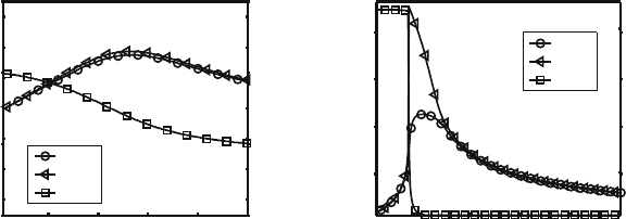
Figure 1 illustrates the evolution of the radiation and material temper-

ature, as well as fuel density of a point near the left boundary. As can be

seen, the high density case yields a very rapid increase in material tempera-

ture and consumes most of the fuel. The low density case results in a slower

evolution of the material temperature. The slowly changing temperature al-

lows for more energy to be transfered to the radiation and loss via diﬀusion.

Since the temperature is lower in this case, a smaller fraction of the fuel is

consumed.

0.01 0.02 0.03 0.04 0.05

0.2

0.4

0.6

0.8

1.2

1.4

Temperature (keV)

time (µs)

0.005

0.01

0.015

Fuel Density (g/cm

)

= 0.01

0.01 0.02 0.03 0.04 0.05

Temperature (keV)

time (µs)

−5

−4

−3

−2

Fuel Density (g/cm

)

= 0.03

Fig. 1. Evolution of radiation temperature, material temperature, and fuel density

for two simulations. Values plotted are for a point near the left boundary. Linear

scale used on the low density case and a log scale used on the high density case

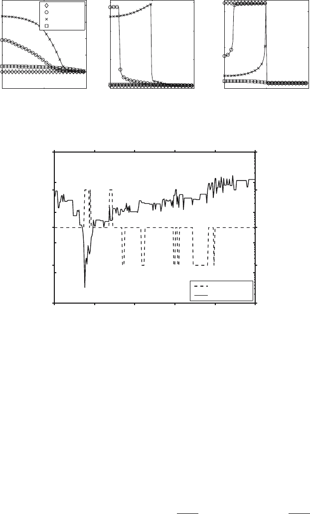
Figure 2 shows proﬁles of radiation temperature, material temperature,

and fuel density at various times for the

F 0

=0.03 g/cm

simulation. Diﬀu-

sion loss of energy results in a lower temperature in the outer region. Thus,

the inner region begins to consume fuel and heat up sooner than the outer

region resulting in a steep temperature gradient that sweeps through the fuel

region (see Fig. 2). These results are similar to the reaction-diﬀusion wave

results presented in the next section.

Figure 3 gives the history of the time step and integration order for the

higher fuel density case. The smallest step size, which occurs during the

rapid heating stage, is 3.26 × 10

−8

µs. The longest time, in the quiescent

period at the end of the simulation, is 5.31 × 10

−4

µs. This large diﬀerence

in step sizes illustrates the ability of our method to select time step size and

integration order resulting in the largest time step possible subject to the

accuracy constraints.

Implicit Solution of Non-Equilibrium Radiation Diﬀusion 361

0510

0.5

1.5

2.5

Radiation Temperature

(keV)

r (cm)

t =0.0002 µs

t =0.0076 µs

t =0.0082 µs

t =0.0598 µs

0510

Material Temperature

(keV)

r (cm)

0510

Fuel Density

(g/cm

)

r (cm)

Fig. 2. Radiation temperature, material temperature and fuel density proﬁles at

various times for the ρ

F 0

=0.03 g/cm

run

0 0.01 0.02 0.03 0.04 0.05

Order

time (µs)

Order

Time Step

−8

−7

−6

−5

−4

−3

Time Step (µs)

Fig. 3. History of time step and integration order

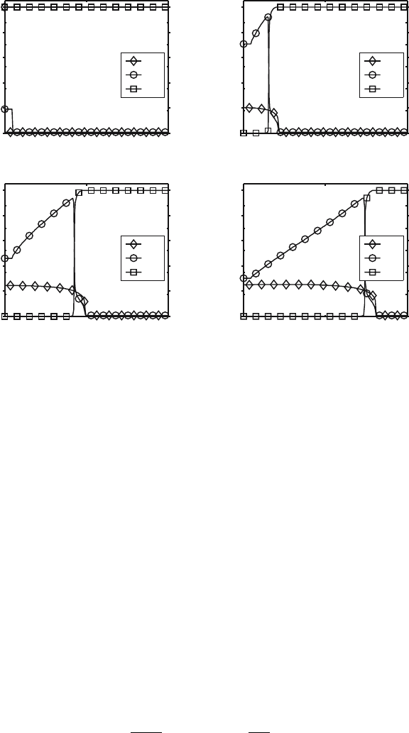
4.2 1D Reaction Diﬀusion Wave

In the previous section we initialized the simulation with a uniform initial

material temperature and a step function for the initial fuel density. The sim-

ulation in this section begins with a uniform fuel density and a step function

in the initial material temperature. These initial conditions produce a reac-

tion diﬀusion wave which is propagated by the diﬀusion of radiation energy

and is driven by the energy from the fusion reaction.

The 1D domain for this simulation is 0.0to2.0 cm, with a uniform fuel

density of 0.1 g/cm

, and uses 200 grid points. The initial background radia-

tion and material temperatures are set to 0.1 keV except for a small region on

the left from 0 to 0.1 cm where the material energy is initialized to 2.0keV.

The reaction parameters are, σ

=1.43×10

sec−g

and e

=1.35×10

erg

sec−g

362 D.E. Shumaker and C.S. Woodward

0 0.5 1

Temperature (keV)

r (cm)

Time = 0.00000 µs

0.02

0.04

0.06

0.08

0.1

Fuel Density (g/cm

)

0 0.5 1

Temperature (keV)

r (cm)

Time = 0.00030 µs

0.02

0.04

0.06

0.08

0.1

Fuel Density (g/cm

)

0 0.5 1

Temperature (keV)

r (cm)

Time = 0.00060 µs

0.02

0.04

0.06

0.08

0.1

Fuel Density (g/cm

)

0 0.5 1

Temperature (keV)

r (cm)

Time = 0.00090 µs

0.02

0.04

0.06

0.08

0.1

Fuel Density (g/cm

)

Fig. 4. Proﬁles at various times for a reaction diﬀusion wave moving from left to

right

This simulation also uses the LEOS equation-of-state data base [13] for hy-

drogen.

The high density region begins to heat much faster than the remainder

of the domain. Diﬀusion of radiation energy heats the material in front of

the wave leading to more heating due to the fusion reactions. Figure 4 gives

proﬁles at four diﬀerent times.

4.3 0D Analytic Test

In this section we demonstrate accuracy of the implicit solution for fusion

heating of the material and the fuel evolution by a comparison with an ana-

lytic solution.

In order to obtain the analytic results, two simplifying assumptions are

made. First, we assume κ

= 0. This assumption eliminates the exchange of

energy between radiation and material and thus removes the radiation energy

equation and diﬀusion from the system. With this assumption the material

energy equation reduces to,

∂E

∂t

= e





. (19)

Implicit Solution of Non-Equilibrium Radiation Diﬀusion 363

Second, the relationship between E

and T

, normally determined by tables

in LEOS, is replaced by the simple linear relation, E

= ρc

,wherethe

speciﬁc heat, c

, is assumed to be a constant.

From the coupled pair of (19) and (3), it can be shown that the sum of

the material energy, E

, and the potential nuclear energy, e

W = E

+ e

, (20)

is independent of time. Thus we can use the conservation relation,

(t)+e

(t)=E

+ e

F 0

, (21)

to eliminate E

(t) from (3), which becomes,

∂

∂τ

= −

(τ)(b − ρ

(τ))

, (22)

where b = E

+ ρ

F 0

and τ = σ

(

ρc

)

t, and where the initial fuel

density and material energy are

F 0

and E

, respectively.

With some help from Mathematica the solution can be expressed as a

transcendental equation,

F 0

)+P (ρ

F 0

) − L(ρ

(τ)) − P (ρ

(τ)) = τ, (23)

where L and P are given by,

(τ)) =

(log(ρ

(τ)) − log(ρ

(τ) − b)) , (24)

and,

P (

(τ)) =

−4b

500

(τ) −

260

(τ)+70bρ

(τ) − 20ρ

(τ)

(b − ρ

(τ))

(τ)

(25)

This analytic result can be used in two diﬀerent ways. We could solve the

transcendental (23) for

(τ) at a number of diﬀerent times, τ , then compare

these values with the computed solution from our code. Or, we could use (23)

to solve for τ when

(τ) is some fraction, α, of the initial value, ρ

(0). We

chose the latter method, since it avoids any computation error associated

with a transcendental solution. The time at which

(τ)=αρ

F 0

is obtained

from (23),

= L(ρ

F 0

)+P (ρ

F 0

) − L(αρ

F 0

) − P (αρ

F 0

) (26)

The τ, and thus t, determined by the above equation, is used to verify

our solution. After we have established the parameters for a test run and

selected a value for α, we use this equation to determine a stopping time

for the simulation. The simulation computes the ﬁnal fuel density, and this

density is then compared to the expected α

F 0

364 D.E. Shumaker and C.S. Woodward

For this test problem we use the following parameters, ρ =1.0 g/cm

=5.755 ×10

erg/keV, e

=1.35 ×10

erg

sec−g

,andσ

=1.43 ×10

sec−g

The initial material temperature is 50.0 keV, and the initial fuel density is

0.1 g/cm

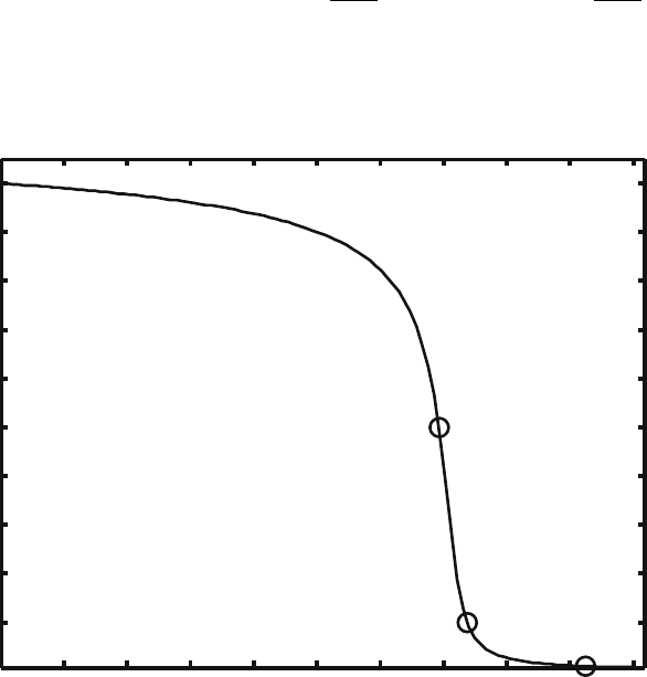
. We chose three values of α, (0.5, 0.1 and 0.01), to determine check

point times. These times are indicated on Fig. 5 which gives the fuel density

versus time for this simulation.

0 0.2 0.4 0.6 0.8 1 1.2 1.4 1.6 1.8 2

x 10

−6

0.01

0.02

0.03

0.04

0.05

0.06

0.07

0.08

0.09

0.1

Fuel Density (g/cm

)

time (µs)

Fig. 5. Evolution of fuel density for 0D analytic comparison test problem. Markers

indicate the compared test values at

=0.5 ρ

(0), ρ

=0.1 ρ

(0) and ρ

0.01

(0)

Table 1 gives the relative error in fuel density for values of RTOL from

−4

to 10

−12

along with the number of time steps, NST. Note that absolute

tolerances were set to equal the relative tolerances. We see that the error

decreases linearly with the RTOL value indicating good convergence of the

implicit solution method. We also see a fairly large increase in the number

of time steps required to resolve the solution for RTOL values less than

−8

. As one would expect, requiring very high accuracy comes at a price in

computation time.

Implicit Solution of Non-Equilibrium Radiation Diﬀusion 365

Table 1. Statistics and Error for 0D Analytic Problem

=0.5ρ

(0) ρ

=0.1ρ

(0) ρ

=0.1ρ

(0)

RTOL NST ERROR NST ERROR NST ERROR

−4

144 −1.01 × 10

−2

159 −2.09 × 10

−2

196 −1.74 × 10

−3

−6

157 −1.65 × 10

−3

177 −3.08 × 10

−3

219 −4.81 × 10

−4

−8

173 −2.79 × 10

−5

217 −5.18 × 10

−5

289 −4.51 × 10

−6

−10

258 −2.93 × 10

−7

359 −5.67 × 10

−7

500 4.72 × 10

−9

−12

484 −9.84 × 10

−9

686 −1.72 × 10

−8

967 −1.87 × 10

−10

NST = time steps

4.4 2D Results

In this section we present results for a 2D problem illustrating the convergence

with respect to reducing tolerances and varying the maximum allowed order

of integration. The simulation domain consists of a square region 1 cm by 1

cm with 50 grid points in each direction. The initial fuel density is centered

at x = y =0.0 with a smooth radial distribution given by,

(x)=0.1 B



+ y

, 0.75



(g/cm

) , (27)

where the bicubic radial distribution, B(x, ), is given by,

B(x, ) ≡

⎧

⎪

⎨

⎪

⎩



+x

2





6 − 8

+x

2



, if − <x≤ 0;



−x

2





6 − 8

−x

2



, if 0 ≤ x<;

0, otherwise .

. (28)

This simulation uses the LEOS equation-of-state data base [13] for hydro-

gen which has a uniform density of 5.0g/cm

. Neumann boundary conditions

are applied at the x =0andy = 0 boundaries. Dirichlet boundary conditions

are applied at x =1andy = 1 where radiation temperature is set to 0.5keV.

Initial Radiation and material temperatures were also set to this value. For

this simulation, the energy per reaction, e

, is set to 1.35 × 10

erg

sec−g

.The

reaction rate ﬁt parameter, σ

,is1.43 × 10

sec−g

as determined for plots

in [16]. The reference temperature, T

,is1keV.

Figure 6 gives the time histories of material and radiation temperatures

and fuel density for the point x =0,y = 0. The material temperature rises

slowly initially; however, the T

dependency in the heating rate leads to

a rapid increase resulting in a nearly complete depletion of the fuel at this

point.

For points in the outer region which have a lower initial fuel density, the

evolution is somewhat diﬀerent. Radiation energy from the hotter central

region passes through this outer region. The parameters for this simulation,