Graebel W.P. Advanced Fluid Mechanics
Подождите немного. Документ загружается.

154 Exact Solutions of the Navier-Stokes Equations
For the case where no inner wall is present, 0 ≤ r ≤ b, and as a approaches zero in
equation (5.3.5), B
k
also approaches zero and equation (5.3.6) becomes J
1
kb =0. A
k
is determined as before, using v
t
r 0 =−v
s
r.
For flow outside a cylinder and extending to infinity b ≤ r ≤, the problem is
not as simple. Since both Bessel functions J
1
and Y
1
go to zero as r goes to infinity,
the condition at infinity is automatically satisfied. Thus, only the condition at the wall
need be imposed, which gives equation (5.3.5).
In this case, rather than a Fourier series solution as in equation (5.3.4), there is a
continuous spectrum of k rather than a discrete one, and the summation over the finite
spectrum is replaced by an integral over a continuous spectrum of ks. The result is
v
t
=e
−k
2
t
0
Ak
Y
1
kaJ
1
kr −Y
1
krJ
1
ka
dk (5.3.7)
where we have implicitly assumed that k is real—that is, that the solution decays
exponentially in time with no oscillations. Ak is again determined by the initial
condition, which this time requires solution of an integral equation. Some zeros of the
Bessel functions have been listed in tables. Others can be found by numerical integration.
5.4 Steady Flows When Convective Acceleration Is Present
There are a few special flows that allow similarity solutions of the full Navier-Stokes
equations even when the convective acceleration terms are present. Generally these
problems involve specialized geometry and are of an idealized nature. These similarity
solutions, even though they are for idealized geometries, do, however, provide much
of our basic understanding of laminar viscous flows. They also serve both as a starting
point, as well as a validation, of approximate and numerical solutions.
Our analysis of these flows starts with a stream function in all cases. To have a
similarity solution, the stream function will generally be of the form = x y U .
Putting this into dimensionless form, it becomes
=
x
n
F
xU
yU
(5.4.1)
where n =0 for two-dimensional problems (Lagrange’s stream function) and n = 1 for
three-dimensional axisymmetric problems (Stokes stream function). Here, U = Ux is
a characteristic velocity of the flow and is generally given by the tangential slip velocity
at the boundary found from an inviscid solution of the problem. In the flows for which
similarity solutions hold, F is generally taken to be of the form
F =
xU
f (5.4.2)
where, reminiscent of Stokes’s first problem, the dimensionless variable is defined by
=
yU
xU
=
y
x
xU
(5.4.3)
This form will reduce the nonlinear partial differential Navier-Stokes equations to a
nonlinear ordinary differential equation, which then usually must be solved numerically.
We can show the application of this with several examples.
5.4 Steady Flows When Convective Acceleration Is Present 155
–6 –4 –2 0 2 4 6
6
5
4
3
y
x
2
1
0
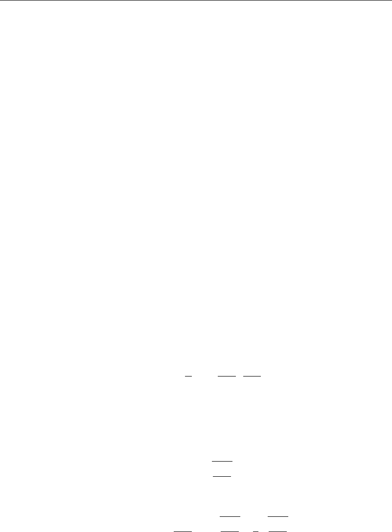
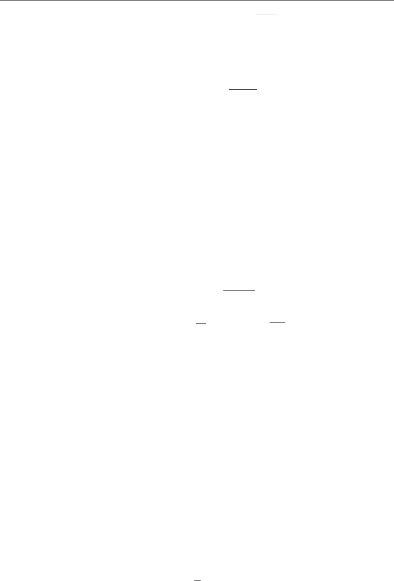
Figure 5.4.1 Streamlines for plane stagnation point flow
5.4.1 Plane Stagnation Line Flow
The flow impinging normally against a plane located at y = 0, with axes set so that
there is a stagnation point at (0,0) as in Figure 5.4.1, was first solved by Hiemenz in
1911. The simplest irrotational flow that corresponds to this case is = axy, with a
slip velocity U = ax on the boundary. The constant a has dimensions of reciprocal
time.
The irrotational flow = axy by itself is not particularly interesting. However,
it is a good model for the stream function in the vicinity of a stagnation point. For
instance, it can be shown to be the local value of the stream function for any flow past
an obstacle—for example, a uniform flow past a circular cylinder.
Taking U = ax as the representative velocity from the preceding, we have from
our general form (5.4.1)
=
xU
f =
ax
2
f or =x
a
f (5.4.4)
where =y
√
a/. We see then that v
x
=/y =axf
v
y
=−/x =−
√
a/f,
where primes denote differentiation with respect to .
The no-slip boundary conditions are that v
x
=v
y
=0aty =0, requiring that f0 =
f
0 = 0. We will also require that v
x
approach U far from the plate, so that f
must
approach 1 as approaches infinity.
The following quantities are needed for use in the Navier-Stokes equations:
v
x
x
=af
v
x
y
=xa
a/f
2
v
x
x
2
=0
2
v
x
y
2
=
xa
2
f
v
y
x
=0
v
y
y
=−af
2
v
y
x
2
=0
2
v
y
y
2
=−a
a/f
156 Exact Solutions of the Navier-Stokes Equations
Notice the following order of magnitude relations for later reference:
O
v
x
v
y
=
x
2
a/ =
xU/ and O
⎛
⎜
⎜
⎝
2
x
2
2
y
2
⎞
⎟
⎟
⎠
=0 (5.4.5)
Here,
√
xU/ is the local Reynolds number for the flow. These orderings will be used
in Chapter 6 in developing the boundary layer approximation.
Substituting the above into the two-dimensional Navier-Stokes equations, we have
axf
af
+
−
a/f
xa
a/f
=−
p
x
+xa
2
f
and
axf
·0+−
a/f −af
=−
p
y
+
−a
a/f
Since we started with a stream function, continuity is automatically satisfied.
Solving for the pressure gradients from the preceding equations, we find that
1
p
x
=xa
2
−f
2
+ff
+f
(5.4.6)
and
1
p
y
=
a/
1
p
=−a
√
aff
+f
(5.4.7)
Again, note for later reference that
O
⎛
⎜
⎜
⎝
p
x
p
⎞
⎟
⎟
⎠
=
Ux/
The second of these equations can be integrated exactly, giving p =−a05f
2
+
f
+ function of x. For now, let the function of x be written as hx. Substituting the
pressure into equation (5.4.6), the result is
dh
dx
=xa
2
−f
2
+ff
+f
Comparing this with equation (5.4.6), we see that the only possibility of having the
variables x and separate is for
h =−05x
2
a
2
A
giving
f
+ff
−f
2
=−A = integration constant (5.4.8)
For the potential flow corresponding to = axy, Bernoulli’s theorem gives the
pressure as
p =−05v
2
x
+v
2
y
=−05a
2
x
2
+y
2
(5.4.9)
5.4 Steady Flows When Convective Acceleration Is Present 157
TABLE 5.4.1 Two-dimensional stagnation point flow against a plate (Hiemenz)
f f
f
f f
f
0000000 00000 12326 2013620 09732 00658
0100060 01183 11328 2215578 09839 00420
0300510 03252 09386 2619538 09946 00156
0400881 04145 08463 2821530 09970 00090
0501336 04946 07583 3023526 09984 00051
0601867 05663 06752 3225523 09992 00028
0702466 06299 05973 3427522 09996 00014
0803124 06859 05251 3629521 09998 00007
0903835 07351 04587 3831521 09999 00004
1004592 07779 03980 4033521 10000 00002
1105389 08149 03431 4235521 10000 00001
1206220 08467 02938 4437521 10000 00000
1307081 08738 02498 4639521 10000 00000
1407967 08968 02110 4841521 10000 00000
1508873 09162 01770 5043521 10000 00000
1609798 09323 01474 5548521 10000 00000
1710737 09458 01218 6053521 10000 00000
1811689 09568 01000 6558520 10000 00000
1912650 09659 00814 7063520 10000 00000
Since far from the wall the condition f
approaches zero implies that f approaches
plus a constant, Bernoulli’s equation and our viscous result for the pressure are seen to
agree far from the wall, providing A is taken to be unity. Then we are left with
xy wall
=
v
x
y
y=0
=xa
a/f
0 = 12326U
2
/
xU/ (5.4.10)
with
f
+ff
−f
2
=−1 (5.4.11)
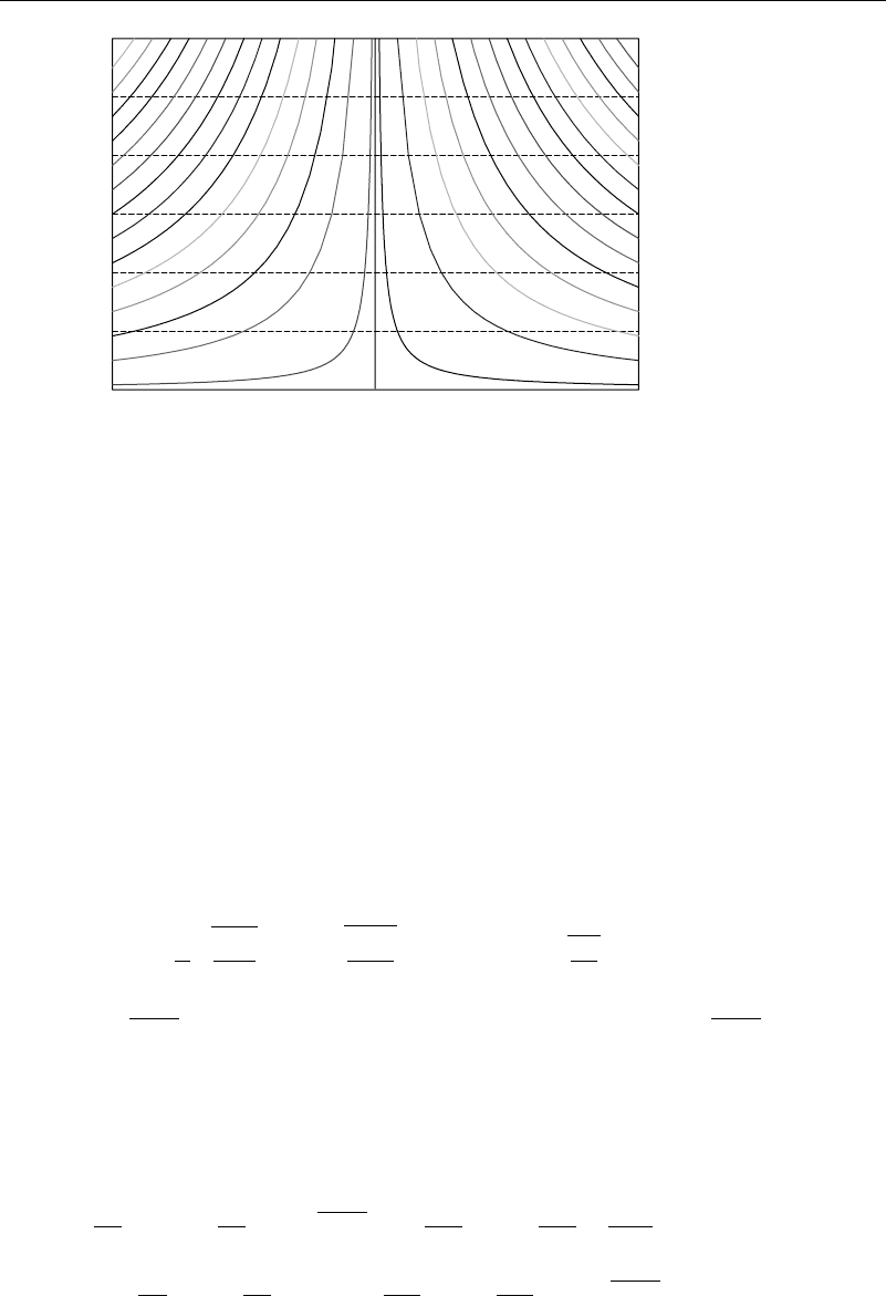
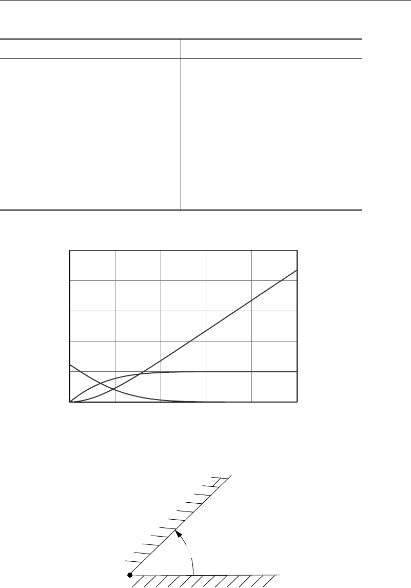
The numerical solution of equation (5.4.8) subject to the boundary conditions was
originally obtained by Hiemenz in 1911 and is given in Table 5.4.1 and Figure 5.4.2.
4
5
3
2
1
01 3
eta
f
′
f
″
f
452
Figure 5.4.2 Hiemenz’s solution for plane stagnation point flow
158 Exact Solutions of the Navier-Stokes Equations
The table shows that for y greater than 24
√
/a, the difference between the
irrotational solution and the Navier-Stokes solution is less than 1 percent. Thus, when
we required our viscous solution to approach the inviscid solution as approached
infinity, this limit was, for practical purposes, achieved at = 24. It follows that a
constant thickness boundary layer exists in this case, with the boundary layer thickness
in the form
=24x/
Ux/ (5.4.12)
Inside this boundary layer, viscosity affects the flow in an important manner. Outside
of this region, viscous effects have a negligible effect on our flow.
5.4.2 Three-Dimensional Axisymmetric Stagnation Point Flow
In 1936 Homann provided a three-dimensional analog of the previous two-dimensional
stagnation point case. This time use
v
r
=−
1
r
z
v
z
=
1
r
r
The axisymmetric potential flow =−ar
2
z will be used as our starting point, since it
has a downward velocity toward the plate of v
z
=−2
ar and a radial velocity of v
r
=az.
Thus, we have U =ar for the slip velocity along the plate and by Bernoulli’s equation
a pressure of
p =−a
2
4r
2
+z
2
2
Again, a is a constant with dimensions of reciprocal time. Letting
=−r
2
√
af =z
a/
we can carry out the calculations in the same manner as in the two-dimensional case.
The final result of these manipulations is the equation
f
+2ff
−f
2
=−1 (5.4.13)
which differs from equation (5.4.8) only by the number 2 multiplying the term containing
the second derivative. The numerical results satisfying the boundary conditions f0 =
f
0 =0f
approaching 1 as gets large, differ little from the preceding case, as can
be seen from Table 5.4.2 and Figure 5.4.3.
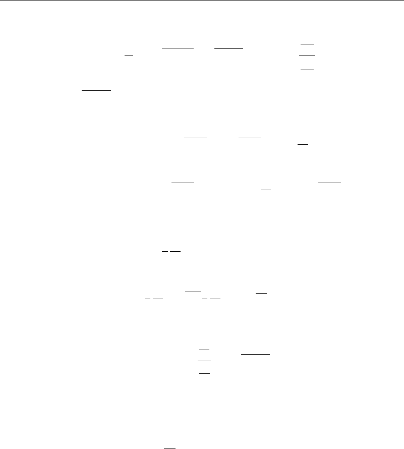
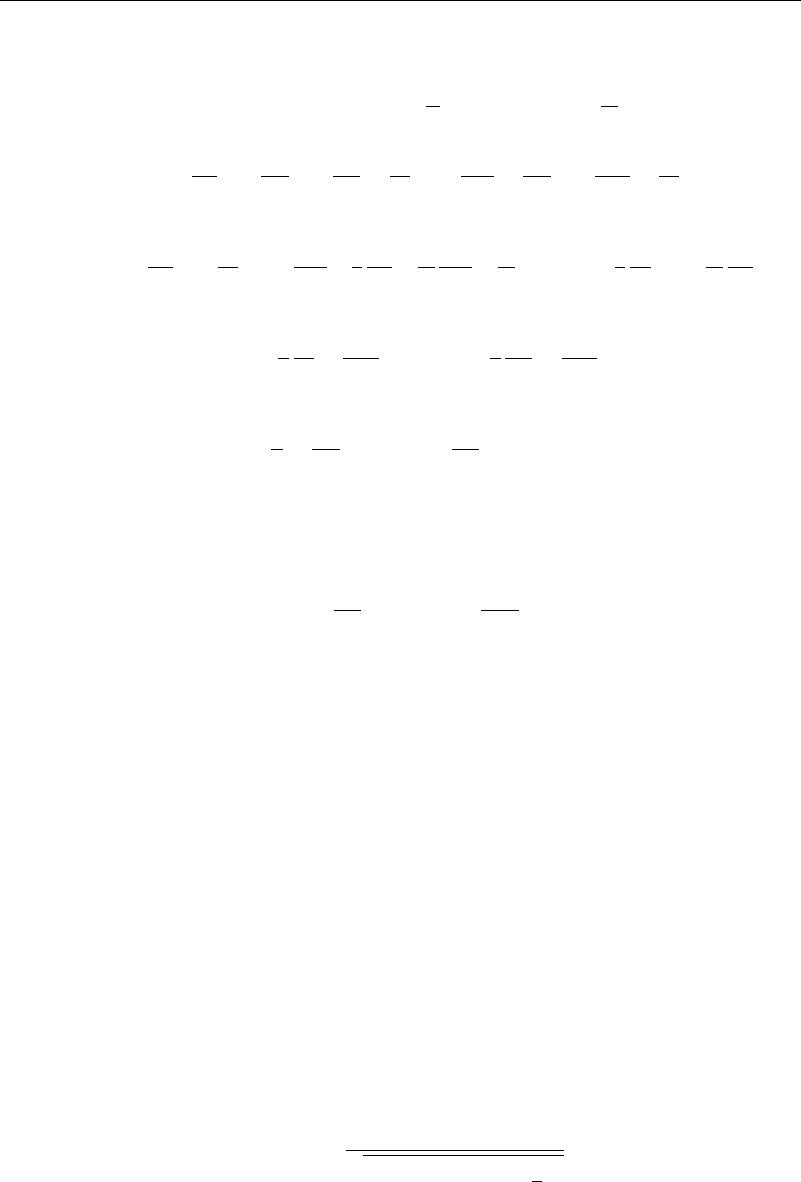
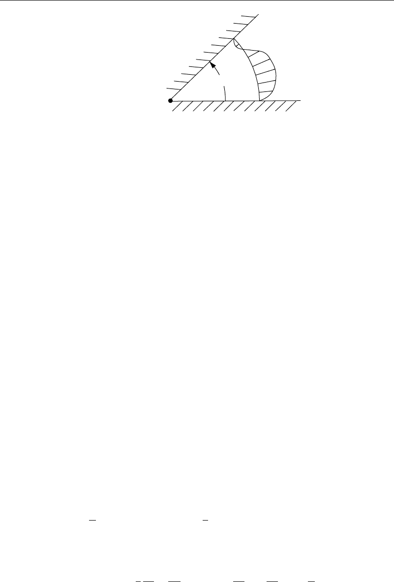
5.4.3 Flow into Convergent or Divergent Channels
One interesting flow that shows a form of flow separation is that between two nonparallel
plates an angle apart, as shown in Figure 5.4.4. This flow was first studied by Jeffrey
(1915) and elaborated further by Hamel (1917). A source or a sink is placed where the
two planes meet. To use our standard form (5.4.2) for the stream function, we work in
cylindrical polar form and recognize that the inviscid flow in this case is like a source or
sink, with streamlines being straight radial lines passing through the source/sink. From
continuity considerations our radial velocity component then is proportional to 1/r, and
the stream function for the channel must therefore be of the form
=
F
Q/
(5.4.14)
5.4 Steady Flows When Convective Acceleration Is Present 159
TABLE 5.4.2 Three-dimensional stagnation point flow against a plate (Homann)
f f
f
f f
f
0000000 00000 13121 1408495 09401 01736
0100064 01262 12121 1509443 09555 01359
0200249 02424 11123 1610405 09675 01046
0300545 03487 10129 1711377 09766 00793
0400943 04451 09147 1812357 09835 00591
0501432 05317 08183 1913343 09886 00433
0602003 06088 07247 2014334 09923 00221
0702647 06767 06347 2216323 09968 00154
0803354 07359 05494 2418319 09989 00072
0904116 07868 04696 2620318 09999 00032
1004925 08300 03961 2822318 09999 00014
1105774 08663 03295 3024319 09999 00007
1206655 08962 02702 3226321 09999 00004
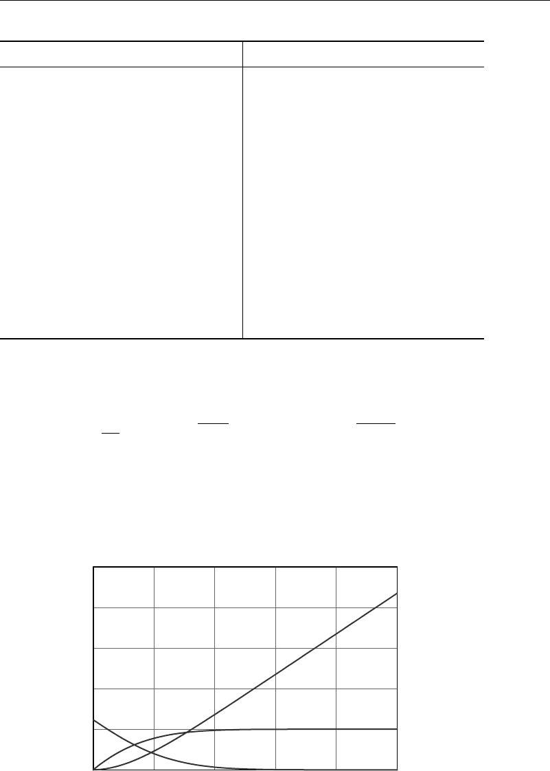
1307564 09205 02182
4
5
3
2
1
01 3
eta
f
′
f
″
f
452
Figure 5.4.3 Homann’s solution for axisymmetric stagnation point flow
α
Source/sink
Figure 5.4.4 Flow in a converging–diverging channel
160 Exact Solutions of the Navier-Stokes Equations
the radial coordinate r dropping out of the list, since it cannot be combined with the other
variables to form a dimensionless parameter. Thus, only a radial velocity component is
present.
This velocity is of the form v
r
=
r
f, with f =
dF
d
, which automatically
satisfies continuity. Using primes to denote differentiation with respect to , find then that
v
r
r
=−
r
2
f
v
r
r
=
r
f
2
v
r
r
2
=
2
r
3
f
2
v
r
r
2
=
r
f
The Navier-Stokes equations in cylindrical polar form in this case are
v
r
v
r
r
=−
p
r
+
2
v
r
r
2
+
1
r
v
r
r
+
1
r
2
2
v
r
2
−
v
r
r
2
0 =−
1
r
p
+
2
r
2
v
r
giving for the pressure gradients
1
p
r
=
2
2
r
3
f
2
+f
1
p
r
=
2
2
2
r
3
f
Integration of these gives
p
=
2
2
r
2
f +hr =−
2
2r
2
f
2
+f
+H (5.4.15)
Comparing terms on the left and right sides of this equation, we can see that hr
has to be of the form
2
A/r
2
, where A is a constant, and H has to be a constant that
can arbitrarily be set to zero. The 1/r
2
dependency of p is consistent with the pressure
field for an inviscid flow far from a source/sink. Thus,
p =
2
r
2
2f +A
=−
2
2r
2
f
2
+f
(5.4.16)
and
f
+f
2
+4f +2A = 0 (5.4.17)
Equation (5.4.17) can be integrated once if we first multiply it by f
. The result is
05f
2
+1/3f
3
+2f
2
+2Af +B = 0 (5.4.18)
where B is a second constant of integration.
Before going further with the solution, consider the boundary conditions. From the
no-slip conditions, f must vanish at both walls of the wedge. Thus, from equations
(5.4.16) and (5.4.18), A =−f
wall
and B =−05f
wall
2
. Unfortunately neither f
wall
nor
f
wall
are known.
We could try to express our constants in terms of the discharge per unit length
into the paper, Q =
rv
r
d =
fd, the integral being over the angle of the wedge.
Q would normally be a given quantity but we would first have to know f to be able to
carry out the integration.
Alternately, we could interpret A in terms of the pressure along a wall, so A =
r
2
p
wall
/
2
, where p
wall
varies like 1/r
2
. This perhaps makes the most sense, as it is
the pressure gradient that drives the flow.
Traditional procedure has been to note that equation (5.4.30) is a first-order equation
and is one where the variables can be separated. This gives
=
df
−2B −4Af −4f
2
−
2
3
f
3
+C (5.4.19)
5.4 Steady Flows When Convective Acceleration Is Present 161
where C is still another constant of integration. The three constants A B, and C are to
be determined such that the no-slip and discharge conditions
f± =0Q=
−
rv
r
d (5.4.20)
where Q would normally be a given quantity.
This solution can be rewritten in the form of elliptic integrals, but the interpretation
of the result is still complicated, since it gives as a function of f rather than vice
versa, and either numerical integration or tables are necessary to interpret the elliptic
integrals. Further, at a point of maximum f the integrand become singular and the sign
of the square root changes.
Two separate approaches have been used to carry out computations of equation
(5.4.19). In 1940 Rosenhead made the substitution
A =−ab +ac +bc/6B=−abc/3 where a +b +c =−6
This enabled him to factor the cubic terms under the square root in equation (5.4.3).
The following conclusions have been reached for various ranges of these constants:
•
If the constant a is real and positive, the constants b and c are complex conjugates
of each other. In this case, the flow will have a positive velocity (sink flow)
throughout.
•
If the constants a b, and c are real, with a>b>c, and a>0 c<b<0, there
can be one or more regions of reversed flow.
•
Rosenhead also found that for a given wedge angle and value of Q/, there is an
infinite number of solutions. Also, for a given number of inflow-outflow regions
and wedge angle there is a critical value of Q/ above which the solution
doesn’t exist.
•
Millsaps and Pohlhausen (1953), using a slightly different approach, made further
calculations and found that for pure outflow problems as Q/ is increased, the
flow concentrates more and more in the center of the wedge.
•
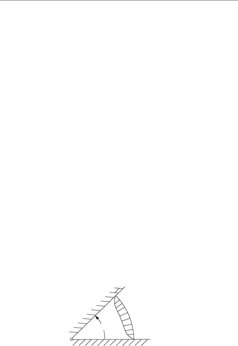
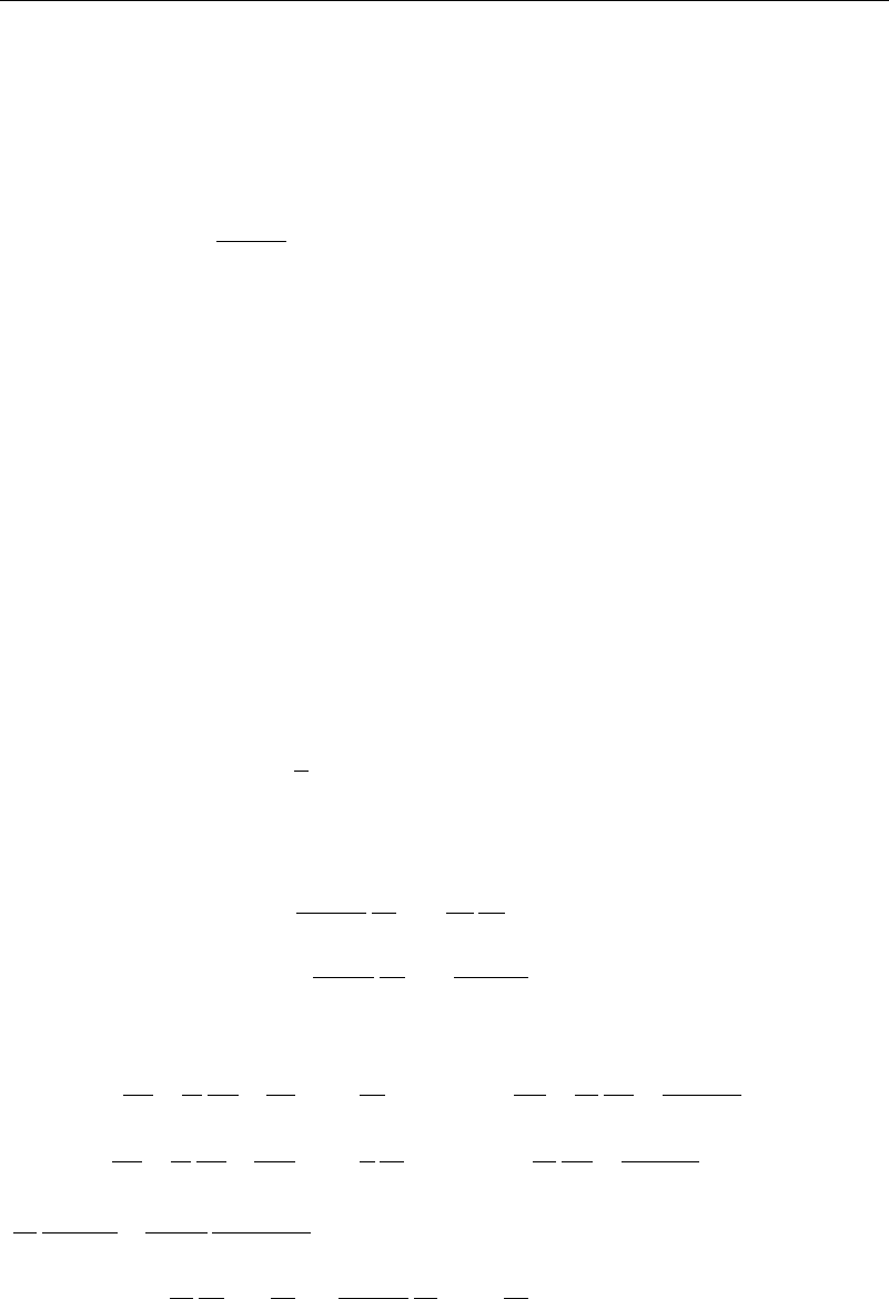
If Q<0 (sink flow), f is symmetric about a center line and always negative.
There is no flow reversal (Figure 5.4.5a).
•
If Q>0 (source flow), too large a value of Q/ for a given wedge angle can
result in unsymmetric flow with reversed flow near one or more walls. The nature
of the flow has to do with the question of whether the roots of the cubic term
under the square root sign in equation (5.4.30) are real or imaginary equation
(Figure 5.4.5b).
α
Sink
Figure 5.4.5a Velocity profile for a converging channel
162 Exact Solutions of the Navier-Stokes Equations
α
Source
Figure 5.4.5b Velocity profile for a diverging channel
•
Most of the simpler two-dimensional flows have three-dimensional counterparts.
Interestingly, this one does not! (Try a radial velocity inversely proportional to
R
2
in spherical coordinates to convince yourself.) This suggests that flow into an
ideal conical funnel must be much more complicated than the simple radial flow
one might expect.
This seemingly simple problem with an exact solution (if you are willing to accept
that elliptic integrals are “well-known functions”) illustrates the complexities that can
arise from solutions of the Navier-Stokes equations.
An alternate approach to the solution of this equation for those who have access to
personal computers involves straightforward numerical integration of equation (5.4.18)
after suitable choice of the constants A and B. Select values for A and B, and then
integrate equation (5.4.18) numerically, using, say, a Runge-Kutta scheme, continuing
the integration until f
becomes zero. You may consider the corresponding angle to
be an acceptable value of the wedge angle, or you may continue if you wish to allow
reversed flow. Numerical integration of f according to equation (5.4.31) will give you
the discharge for your choice of parameters. Since there are no square roots in this
procedure, it is not necessary to test for signs or patch solutions together.
If you want your constants to give a pure source flow, the integration should proceed
until f
becomes zero, which would be at the location of the center line of the wedge.
The flow past the center line is a mirror image of this flow. After you have done many
computations for values of the constants, you should have a better understanding of
these flows.
5.4.4 Flow in a Spiral Channel
Hamel also considered flow into a channel, which is in the shape of a logarithmic spiral
whose shape is given in cylindrical polar coordinates by A +B ln r = constant. Like
the approach in the previous section, he let
=
f and p = p
0
+
r
2
P(), where =A +B ln r (5.4.21)
Letting primes denote differentiation with respect to , the radial and theta velocity
components are
v
r
=
1
r
=
A
r
f
v
=−
r
=−
B
r
f
=−
B
A
v
r
5.4 Steady Flows When Convective Acceleration Is Present 163
Substitution of these into the Navier-Stokes equations leads to
−2P +BP
=
A
2
+B
2
f
2
+Af
AP
=
A
2
+B
2
2f
−Bf
(5.4.22)
From these the pressure is found to be
P =
A
2
+B
2
2A
−A
f
2
+2Bf
−A
2
+B
2
f
(5.4.23)
and the governing equation for the stream function is
A
2
+B
2
f
iv
−4Bf
+4 +2Af
f
=0
This can be integrated once to give
A
2
+B
2
f
−4Bf
+4 +Af
f
=c
1
(5.4.24)
which is second order in f
. The boundary conditions are that f
vanish on the walls—
say, =0 and
1
. The remainder of the solution procedure is much the same as in the
previous section.
5.4.5 Flow Due to a Round Laminar Jet
The solution for the round laminar axisymmetric jet was first presented by Landau
(1944) and later rediscovered by Squire (1951). Working in spherical coordinates they
considered a (vanishing) thin tube injecting fluid at the origin with a stream function
=
Rf where = cos (5.4.25)
(The use of cos rather than itself simplifies the following equations considerably.)
Then the velocity components are given by
v
R
=
1
R
2
sin
=−
R
df
d
v
=−
1
R sin
R
=−
f
R sin
(5.4.26)
For axisymmetric flow the Navier-Stokes equations are
v
R
v
R
R
+
v
R
v
R
−
v
2
R
=−
p
R
+
2
v
R
−
2v
R
R
2
−
2
R
2
v
−
2v
cot
R
2
v
R
v
R
+
v
R
v
+
v
R
v
R
=−
1
R
p
+
2
v
+
2
R
2
v
R
−
v
R
2
sin
2
1
R
2
R
2
v
R
R
+
1
R sin
v
sin
=0
where
2
=
1
R
2
R
R
2
R
+
1
R
2
sin
sin
(5.4.27)