Graebel W.P. Advanced Fluid Mechanics
Подождите немного. Документ загружается.

124 Surface and Interfacial Waves
To analyze this situation, consider the sum of two sine waves of equal amplitude
and nearly equal wave length, and observe the change in the envelope of the resulting
wave. Let
=A sinkx −t +A sin
k +kx − +t
=2A cos05kx −t sin
k +05kx − +05t
(4.2.1)
This has the appearance of an envelope that looks much like a slowly traveling wave
of wavelength =/k that encloses a much more rapidly traveling wave of wave-
length = 2/k. In the limit, as the wave numbers approach each other, the speed of
propagation of the envelope is then
c
g
=
d
dk
=
d
kc
dk
=c +k
dc
dk
=c −
dc
d
(4.2.2)
The quantity c
g
is called the group velocity.
In the previous section we saw that the general formula for c as a function of wave
number was given by equation (4.1.15) as
c =
k
=
1
k
g +k
2
tanh kh
Thus, for these waves the group velocity is given by
c
g
=
g +3k
2
tanh kh +kh
g +k
2
sech
2
kh
2
k
g +k
2
tanh kh
(4.2.3)
For large wavelengths compared to the depth this is approximated by
c
g
≈
g +3k
2
2
k
g +k
2
(4.2.4)
whereas for long waves, where surface tension effects are small 2
√
/g,
c
g
≈
1
2
g
k
1
2
c (4.2.5)
There are at least two ways for explaining the concept of group velocity. Since
the group velocity is smaller than the wave velocity, the waves advance within their
envelopes until they approach the neck, or nodal point, at the right of the envelope.
As they approach that point, they are gradually extinguished and replaced by their
successors that are formed on the right side of the following node. The waves are thus
“grouped” within the necks of their envelope.
Another explanation of group velocity has to do with the speed at which the
energy of the wave travels. The rate at which work is done on a section of the fluid is
0
−
p
x
dy. The only part of the Bernoulli equation that contributes to the work in the
4.3 Waves at the Interface of Two Dissimilar Fluids 125
linearized theory is
t
. Thus, taking the velocity potential from equation (4.1.15) in the
abbreviated form =e
ky +ikx −ct
(no uniform stream) results in
0
−
p
x
dy =
0
−
t
x
dy =
1
2
ck
2
cos
2
kx −ct (4.2.6)
where the real part of the integrand has been used. Averaging this over a wavelength
gives
1
2
ck
2
2
=
1
2
c
2
. The kinetic energy passing through the section is
1
2
0
−
x
2
dy =
1
2
0
−
ike
ky +ikx−ct
2
dy =
1
4
k
2
cos
2
kx − ct (4.2.7)
which when averaged over the same period gives
1
4
k
2
2
=
1
4
2
. Thus, the kinetic
energy is moved through the fluid at only one-half the wave speed c, which corresponds
to the group velocity.
4.3 Waves at the Interface of Two Dissimilar Fluids
Following the procedure described in the previous section, the theory of waves at an
interface can also be developed. This time consider two fluids: the upper one y > 0
moving with a velocity U
1
and the lower one y ≤ 0 moving with a velocity U
2
. The
investigation will be to determine whether a small disturbance introduced at the interface
will either grow or decay. To accomplish this, choose a flow plus a disturbance in the
form of a progressive wave such that
=
1
=xU
1
+C
1
e
−ky +ikx −ct
for y>0
2
=xU
2
+C
2
e
ky +ikx −ct
for y ≤0
(4.3.1)
Notice that both of these velocity potentials satisfy the Laplace equation. They represent
waves that are traveling in the positive x direction whose amplitude dies out away from
the interface. The (real) parameter k is the wave number and is twice pi divided by
the wave length. The real part of c is the wave speed, and the imaginary part of kc
is the growth rate. If Imag (kc) is positive, the wave will grow, whereas if it is negative
the wave decays. Neutral stability is obtained if c is real.
The form of the interface disturbance that is suited to these potentials is =
Ae
ikx −ct
and the appropriate boundary conditions to be imposed at y =0 are
D
Dt
=
n
and p
2
−p
1
=
R
(4.3.2)
where is the surface tension and R is the radius of curvature of the interface.
As we saw in Section 4.1, imposing nonlinear boundary conditions on an unknown
boundary is a very difficult task. Instead, again assume that the disturbance is very
small—so small, in fact, that nonlinear terms can be neglected—and also that these
boundary conditions can be applied at the undisturbed interface. This will tell us whether
or not a small disturbance will grow. It does not say what happens if growth occurs. In
fact, it says the growth will be unbounded. Obviously, the nonlinear terms will become
important long before that, and in that situation a nonlinear analysis must be used.
126 Surface and Interfacial Waves
Our linearized boundary conditions to be applied then on y =0 are
t
+U
1
x
=
1
y
t
+U
2
x
=
2
y
and
p
2
−p
1
=
2
2
t
+U
2
2
x
+g
−
1
1
t
+U
1
1
x
+g
=
2
x
2
(4.3.3)
The radius of curvature has been linearized here according to
1
R
=
d
2
y
dx
2
1+
dy
dx
2
3/2
≈
d
2
y
dx
2
Substitution of our velocity potentials into this and removing multiplying terms gives
ikU
1
−cA =−kC
1
ikU
2
−cA = kC
2
2
ik
U
2
−c
C
2
+gA
−
1
ik
U
1
−c
C
1
+gA
=−k
2
A
(4.3.4)
Eliminating the C
1
C
2
, and A and solving for c gives
2
−k
U
2
−c
2
+g−
1
k
U
1
−c
2
+g =−k
2
or finally
c =
1
U
1
+
2
U
2
1
+
2
±
g
2
−
1
+k
2
k
1
+
2
−
1
2
U
1
−U
2
2
1
+
2
2
1/2
(4.3.5a)
We can also write this as
c = c
0
±c
1
where c
0
=
1
U
1
+
2
U
2
1
+
2
and c
1
=
g
2
−
1
+k
2
k
1
+
2
−
1
2
U
1
−U
2
2
1
+
2
2
1/2
(4.3.5b)
To decide on the stability of this flow note that c
0
is always real and positive. If
the flow is to be unstable, it must be c
1
that is imaginary. That would occur provided
U
1
−U
2
2
>
g
2
2
−
2
1
+k
2
1
+
2
1
2
k
(4.3.6)
We can see that surface tension is always a stabilizing influence, but for long waves
(small values of k) its effect loses significance. Having a denser fluid on top of a lighter
fluid is of course always destabilizing.
Helmholtz pointed out that where U
1
= U
2
1
=
2
can be used to explain the
flapping of sails and flags. In this case c
1
vanishes, and our solution procedure fails
because of the double root. Repeating the analysis for this special case would be the
same except for the expression for , which now would have to include a time to the
power one multiplier. A disturbance introduced at the edge of a sail or flag would then
grow as it travels along the flag, a frequently observed phenomenon.
The difference in velocities on either side of the interface means that the interface
can be considered as a concentrated vortex sheet. To see this, suppose that rather than
having a discrete jump, the undisturbed flow was given by a velocity profile such as
4.4 Waves in an Accelerating Container 127
U =
U
1
+U
2
2
+
U
1
−U
2
2
tanh
y
. In the limit as gets small this approaches the discontinuous
profile. It has the vorticity component
dU
dy
=
U
1
−U
2
2 cosh
2
y
. Vortices have a tendency to
roll up, as exhibited in the nature of the displacement of the interface.
4.4 Waves in an Accelerating Container
Transportingaliquidinamovingcontainerisavery effective way of causingsurfacewaves,
as anyone who has carried a cup of coffee across a room has experienced. In transporting
oil across the oceans in large tankers, the breaking of these waves against the bulkheads
can easily create substantial damage. Even in airplanes, as fuel tanks empty the sloshing of
the fuel can create problems. One solution is to break up the surface into smaller regions by
floating dividers, but this leads to difficulties in cleaning the tanks.
Different types of container motion lead to different mechanisms of wave generation.
One of these—waves due to an acceleration in the vertical direction—is examined next.
Consider a rectangular tank of liquid subjected to a translational acceleration in the
vertical direction. Neglect surface tension effects. The liquid will be taken to originally
be in the rectangular region 0 ≤ x ≤ a 0 ≤ y ≤ b −h ≤ z ≤ 0, where the coordinate
system is fixed to the tank. The velocity potential then satisfies the Laplace equation
together with the boundary conditions
x
x =0
=
x
x =a
=0
y
y =0
=
y
y =b
=0
z
z =−h
=0
t
=
z
z =0
t
z=0
+
g +
dV
z
dt
=0
(4.4.1)
The solution of the Laplace equations that satisfies the boundary conditions at the walls
is of the form
=
m =0
n =0
dA
mn
dt
cos
mx
a
cos
my
b
cosh rz +h (4.4.2)
and
=r
m =0
n =0
A
mn
cos
mx
a
cos
my
b
sinh rh (4.4.3)
where r =
m
2
a
2
+
n
2
b
2
. This solution also satisfies the kinematic condition at the free
surface.
The pressure condition at the free surface requires that
d
2
A
mn
dt
2
+r
g +
dV
z
dt
A
mn
tanh rh =0 (4.4.4)
Next introduce the circular frequency
2
=rg tanh rh and take V
z
=−V
0
sin t.
Make time dimensionless by choosing T =
1
2
t and introduce dimensionless parameters
a =
2
2
2q =
V
0
g
2
2
128 Surface and Interfacial Waves
30
25
20
unstable
unstable
unstable
unstable
unstable
a
unstable
unstable
unstable
unstable
15
10
5
0
–5
–10
–15 –10 –5 0
q
51015
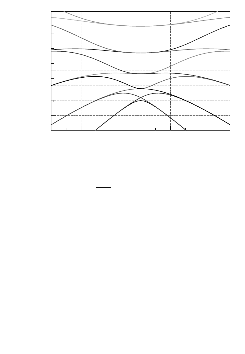
Figure 4.4.1 Strutt diagram
Equation (4.4.4) then becomes
d
2
A
mn
dT
2
+
a −2q cos 2T
A
mn
=0 (4.4.5)
This is the standard form of the Mathieu equation,
1
which has been well studied,
particularly by Rayleigh. He showed that regions of stability were governed by com-
binations of the parameters p and as shown in Figure 4.4.1. This figure is called
the Strutt diagram. If the parameter pair (a, q) lie in a region not labeled, the solution
is oscillatory but not periodic. This nonperiodicity of the wave is an example of the
“weakness” of this type of wave. If the pair p lie in a region labeled unstable, at
least one of the solutions will increase without limit with increasing time.
The lines separating the stable-unstable regions in Figure 4.4.1 are lines along
which one of the solutions is periodic with period 2/, where is the largest integer
with p as an upper bound. The other solution increases in time without bound. Thus,
these dividing lines are considered part of the unstable region. Further information on
the computation of these lines is given in the Appendix.
4.5 Stability of a Round Jet
Liquid jets have a number of industrial applications, including the production of a stream
of droplets. In the early days of the development of the inkjet printer two technologies
were considered. The first one used jet breakup to produce a steady stream of electri-
cally charged droplets, which then were steered by electric fields to either write on a
1
This equation is also encountered in analyzing certain mechanical vibrations, including the inverted
pendulum and the pendulum of varying length.
4.5 Stability of a Round Jet 129
page or to be collected and subsequently recirculated. The second approach, the “drop-
on-demand,” produced individual droplets all of which struck the page. It is the tech-
nology most frequently used today for home printers.
Modern “airless” paint sprayers used for painting automobiles depend on a rotating
cone to throw off a series of jets, each of which rapidly break up into droplets. The
water-based paint is electrically charged as it enters the cone, and an electric potential
between the cone and the item to be painted steers the paint to the target.
The breakup of a liquid jet was first studied by Raleigh in 1876. For a jet of
radius a traveling at a speed U , the velocity potential for the disturbed flow is taken
as =
1
re
ikz +s +t
. This is in the form of a wave traveling along the jet moving
at a speed c. The dependence has been selected so that traveling around the jet
circumference returns us to the starting point. The z dependence gives a wavelike shape
in the z direction.
Inserting this form into the Laplace equation gives
2
=
2
r
2
+
1
r
2
r
2
+
1
r
2
2
2
+
2
z
2
= e
ikz +n +t
d
2
dr
2
+
1
r
d
2
dr
2
−
n
2
r
2
−k
2
1
=0
(4.5.1)
The operator acting on
1
is of the Bessel type. The solution that is finite within the jet
is
1
=AI
n
kr, where I
n
kr is a modified Bessel function given by the series
I
n
kr =i
−n
J
n
ikr =i
−s
m =0
−1
m
m!m +n +1
ikr
2
s +2m
=
kz
2
n
m =0
1
m!m +n +1
kr
2
2m
(4.5.2)
The boundary conditions to be satisfied on the free surface are
t
+U
z
=
r
on r = a
and
p −p
0
=−
t
−U
z
=
1
R
1
+
1
R
2
−
a
=
−
1
a
2
+
2
2
−
2
z
2
on r =a
The kinematic condition gives
=
−i
kU +
d
1
dr
r =a
e
ikz +n +t
=
−ikA
kU +
dI
s
d
=ka
e
ikz +n +t
(4.5.3)
The pressure condition gives
−iAkU +I
s
ka e
ikz +n +t
=
ikA
kU +
1
a
2
dI
s
d
=ka
n
2
+a
2
k
2
−1
e
ikz +n +t
or
kU +
2
=
a
3
kaI
s
ka
I
s
ka
n
2
+a
2
k
2
−1
(4.5.4)
There is thus a possibility that the right-hand side of equation (4.5.4) can be zero
in the range 0 <ka<1. This is a case where the wavelength is greater than the
circumference of the jet. The right-hand side takes its largest negative value when
130 Surface and Interfacial Waves
k
2
a
2
= 04858, or when the wavelength equals = 2/k = 4508 ×2a. Thus, the jet
takes on a series of enlargements and contractions with continually increasing amplitude,
until it breaks up into a series of separated drops.
4.6 Local Surface Disturbance on a Large Body
of Fluid—Kelvins Ship Wave
The waves caused by creating a local disturbance to the surface of a large body of fluid
is of interest in studying the wave pattern associated with ships. Considering the fluid to
be very deep and linearizing the boundary conditions as before, the basic equations are
2
=0 for −≤z ≤ 0
p
=−
t
−g on z = 0 (4.6.1)
t
=
z
on z =0
Working in cylindrical polar coordinates and assuming independence of the angle ,
separation of variables gives
rzt=Ate
kz
J
0
kr J
0
kr =
j =0
−1
j
j!
2
kr
2
2j
(4.6.2)
where J
0
kr is the Bessel function of order zero. Inserting equation (4.6.2) into the
boundary conditions gives
=−
1
g
t
z =0
=
1
g
dA
dt
J
0
kr and
t
=
z
z =0
=kAJ
0
kr (4.6.3)
Having in mind a problem where there is an initial displacement given to the free surface
at r = 0, choose as a solution the forms
r z t =fk
g
k
e
kz
sin
gktJ
0
kr r t =fk cos
gktJ
0
kr (4.6.4)
To find the nature of this solution, first consider a very basic initial disturbance
where the solution is concentrated near the origin. This is a disturbance much like our
Green’s functions of Chapter 2, or like concentrated loads in elementary beam theory,
and is akin to a Dirac delta function. Use the property of integral transforms that
fk =
0
frJ
0
kr2rdr and fr =
1
2
0
faJ
0
arada (4.6.5)
and choose the initial disturbance to be
fr =
⎧
⎨
⎩
lim
a→0
1
a
2
for 0 ≤ r ≤a
0 for a<r
4.6 Local Surface Disturbance on a Large Body of Fluid—Kelvins Ship Wave 131
Then lim
a→0
0
fr2rdr = 1 and
r z t =
0
g
k
e
kz
sin
gktJ
0
krkdk
0
faJ
0
kaada
=
0
g
k
e
kz
sin
gktJ
0
krkdk (4.6.6)
r t =
0
cos
gktJ
0
krkdk
0
faJ
0
kaada
=
0
cos
gktJ
0
krkdk (4.6.7)
It is not possible to evaluate these integrals in closed form. However, if in the
expression for the displacement the cosine is expanded in a Taylor series, it is found that
r t =
1
2r
2
1
2
2!
gt
2
r
−
1
2
·3
2
6!
gt
2
r
3
+
1
2
·3
2
·5
2
10!
gt
2
r
5
−···
(4.6.8)
This tells us that for any particular phase of the displacement, the quantity gt
2
/r is
constant. Thus, the waves travel radially out from where they originated, each phase
traveling with a constant acceleration.
The more important problem would be to determine what the wave pattern would
be as the source moves, emitting wave pulses along the way. That would involve
superposition of the preceding solution over a time integral. The problem was first solved
by Kelvin (1891) using the method of stationary phase that he had in fact originated.
The paper, however, leaves out many details and does not tell how he performed the
analysis. Lamb (1932, §256) provides a figure, but, again, the presentation is sketchy and
difficult to follow. Later papers by Peters (1949) and Ursell (1960) clarified the details
omitted by the previous authors. In any case, the mathematics at this point involves
quite complicated use of asymptotic methods and becomes very involved. Details are
left to the discussions in Lamb, Ursell, and Peters.
Using the notation of Peters, the results can be summarized as follows:
•
The waves are contained within an angle of 2 ·sin
−1
1
3
=38
56
.
•
Two wave patterns exist within this triangle: a set of transverse waves and a set
of divergent waves. The patterns of constant phase are shown in Figure 4.6.1.
They are given by the following:
Transverse waves
g
c
2
rh
1
=
2n +
1
4
n > 0 (4.6.9)
Divergent waves
g
c
2
rh
2
=
2n +
3
4
n > 0 (4.6.10)
Here, r and are the usual cylindrical coordinates centered at the present location
of the disturbance, and c is the speed at which it travels. The various functions
are given by
h
i
=sin coth p
i
cosh
2
p
i
(4.6.11)
with sinh p
1
=
1
4
cot −
√
cot
2
−8 sinh p
2
=
1
4
cot +
√
cot
2
−8.
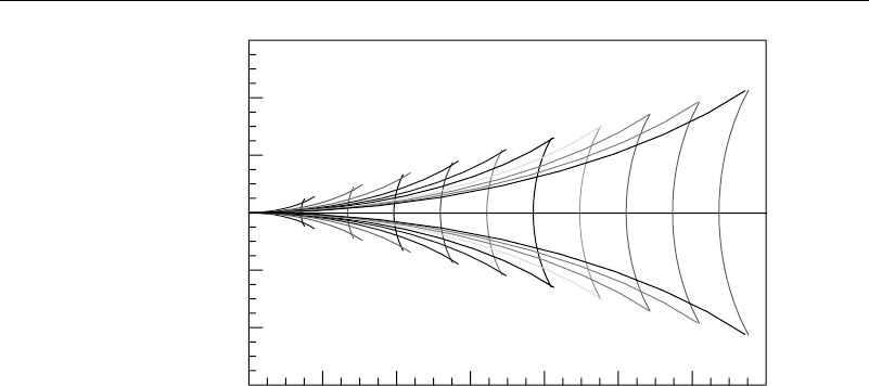
132 Surface and Interfacial Waves
Y
X
30
20
10
0
–10
–20
–30
010203040506070
Figure 4.6.1 Kelvin ship wave—waves of constant phase
The p
i
’s are real if cot
2
≥ 8—that is, −1947
≤ ≤1947
. Outside of this
region the disturbance is greatly diminished.
The preceding pattern is a reasonable depiction of the bow wave on a slender ship or
the pattern due to a tree branch or fish line in the water. Understanding the pattern also
has a practical use. Resistance to the motion of ships is about equally divided between
viscous shear and wave drag. (The waves have a considerable amount of potential
energy, all provided by the ship.) Simple models of a ship use a single source-sink
pair—the source modeling the ship’s bow—to generate the pattern given above. In the
1950s Inui (1957) and others discovered that if somehow another “source” could be
placed in front of the ship’s bow, it could create waves out of phase with the bow wave
and thus cancel them. Experiments conducted in the towing tank at The University of
Michigan by Inui and others confirmed this theory, leading to the now-famous bulbous
bow. This is an underwater rounded protuberance extended from the bow. This idea
was embraced by the world’s tanker fleet, which added bulbous bows and midsections
to existing tankers, enabling greater capacity using the original power supplies. Similar
wave-cancellation ideas are used in noise-cancelling headphones.
4.7 Shallow-Depth Free Surface Waves—Cnoidal
and Solitary Waves
Many years ago, Russell (1838, 1894) pointed out that for wavelengths that were large
with respect to the depth, waves are observed for which shape changes only occur very
gradually as the wave proceeds along a shallow channel. The wave height of these waves
is not necessarily small. To investigate this situation, consider a two-dimensional case
where the wave pattern varies along the channel but not with the direction transverse to
the channel walls. To make the wave pattern steady, the undisturbed flow in the channel
is taken to move at a speed c, this speed being whatever is necessary to make the wave
pattern stationary.
4.7 Shallow-Depth Free Surface Waves—Cnoidal and Solitary Waves 133
First, consider a periodic wave pattern in an infinitely long channel. The x-axis is
taken as being the direction of wave propagation, and the coordinate origin is at the
bottom of the channel. The governing equations and boundary conditions are
2
x
2
+
2
y
2
=0
y
=0ony =0 (4.7.1)
x
x
=
y
and
1
2
x
2
+
1
2
y
2
+g = C on y =
Here, C is a constant that represents the total energy at a point, to be determined later.
Next, following Lamb (1932, §252), assume that a solution can be found for the
velocity potential in the form of a Taylor series in y. Then to satisfy the Laplace
equation, let
x y = G −
y
2
2!
G
+
y
4
4!
G
∓··· (4.7.2)
where G is a function of x and primes denote x derivatives.
Substituting equation (4.7.2) into the boundary conditions gives
G
−
2
2!
G
+
4
4!
G
∓···
=−G
+
3
3!
G
∓···
G
−
2
2!
G
+
4
4!
G
∓···
2
+
−G
+
3
3!
G
∓···
2
=2C −2g
(4.7.3)
At this point, since long waves are being considered, assume that the more G is
differentiated, the smaller its effect becomes. Then, under this assumption, equation
(4.7.3) becomes after rearrangement
G
+G
−
2
2!
G
−
3
3!
G
∓···=0
−2C +2g +
G
2
+
−G
2
−
2
G
G
±···=0
(4.7.4)
The first of these can be integrated, giving
G
−
3
3!
G
±···=D or GF
=
D
+
2
3!
G
∓··· (4.7.5)
where D is a constant of integration. Inserting this into the pressure condition and
simplifying gives
−2C +2g
D
2
+
1
2
+
2
3
−
2
3
2
=0 (4.7.6)
Equation (4.7.6) is a form of the Korteweg-deVries equation (1895). It can be
integrated by first multiplying by
. The result is
−2C +g
2
D
2
−
1
+
2
3
=H (4.7.7)
where H is still another constant of integration.