Gockenbach M.S. Partial Differential Equations. Analytical and Numerical Methods

58

Chapter

3.

Essential

linear

algebra

is

orthonormal,

as can be

verified

directly.

If

3.4.1

The L

2

inner

product

We

have seen

that

functions

can be

regarded

as

vectors,

at

least

in a

formal sense:

functions

can be

added together

and

multiplied

by

scalars. (See Example

3.4 in

Section 3.1.)

We

will

now

show more directly

that

functions

are not so

different

from

Euclidean vectors.

In the

process,

we

show

that

a

suitable inner product

can

be

defined

for

functions.

Suppose

we

have

a

function

g G

C[a,

b]—a

continuous function defined

on the

interval

[a,

&].

By

sampling

g on a

grid,

we can

produce

a

vector

that

approximates

the

function

g. Let Xi = a +

iAx,

A#

= (b

—

a)/N,

and

define

a

vector

G G

R

N

by

Refining

the

discretization (increasing

N)

leads

to a

sampled function

that

obviously

represents

the

original function more

accurately.

Therefore,

we

ask:

What

happens

to F • G as N

->•

oo?

The dot

product

does

not

converge

to any

value

as N

—>•

oo, but a

simple modification induces

convergence.

We

replace

the

ordinary

dot

product

by the

following

scaled

dot

product,

for

which

we

introduce

a new

notation:

Then

G can be

regarded

as an

approximation

to g

(see Figure 3.3). Given

another

function

f(x)

and the

corresponding vector

F €

R

N

,

we

have

bra

58

Chapter

3.

Essential linear algebra

is orthonormal,

as

can

be

verified directly.

If

then

3.4.1 The

L2

inner product

We

have seen

that

functions can be regarded as vectors,

at

least in a formal sense:

functions can be added together and multiplied by scalars. (See Example 3.4 in

Section

3.1.)

We

will now show more directly

that

functions are not so different

from Euclidean vectors. In the process,

we

show

that

a suitable inner product can

be defined for functions.

Suppose

we

have a function 9 E

era,

b]-a

continuous function defined on

the

interval

[a,

b].

By sampling 9 on a grid,

we

can produce a vector

that

approximates

the

function

g.

Let

Xi

= a +

i~x,

~x

=

(b

-

a)/N,

and define a vector G E RN by

Gi=g(Xi),

i=O,l,

...

,N-1.

Then G can be regarded as

an

approximation to 9 (see Figure 3.3). Given another

function

f(x)

and the corresponding vector

FERN,

we

have

N-l

F·G=

L FiGi

i=O

N-l

= L f(xi)g(x;).

i=O

Refining the discretization (increasing

N)

leads

to

a sampled function

that

obviously

represents

the

original function more accurately. Therefore,

we

ask:

What

happens

to

F . G as N

-t

oo?

The dot product

N-l

F . G = L f

(Xi)

9

(Xi)

i=O

does not converge to any value as N

-t

00,

but

a simple modification induces

convergence.

We

replace

the

ordinary dot product by

the

following scaled dot

product, for which

we

introduce a new notation:

N-l

(F,

G) = L

FiGi~X,

i=O

3.4. Orthogonal

bases

and

projections

59

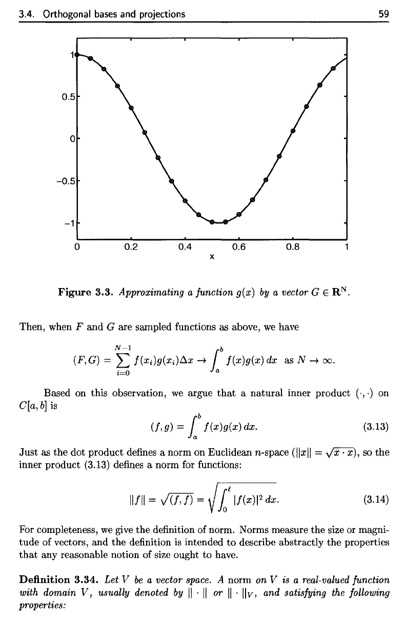
Figure

3.3. Approximating

a

function

g(x]

by a

vector

G €

R

N

.

Then, when

F and G are

sampled

functions

as

above,

we

have

Based

on

this observation,

we

argue

that

a

natural

inner product

(•, •) on

C[a,

b]

is

Just

as the dot

product

defines

a

norm

on

Euclidean

n-space

(\\x\\

=

^/x

•

x],

so the

inner

product (3.13)

defines

a

norm

for

functions:

For

completeness,

we

give

the

definition

of

norm. Norms measure

the

size

or

magni-

tude

of

vectors,

and the

definition

is

intended

to

describe abstractly

the

properties

that

any

reasonable notion

of

size

ought

to

have.

Definition

3.34.

Let V be a

vector

space.

A

norm

on V is a

real-valued

function

with

domain

V,

usually

denoted

by \\ • \\ or \\ •

\\v,

and

satisfying

the

following

properties:

3.4. Orthogonal bases and projections

59

o

0.2

0.4 0.6

0.8

x

Figure

3.3.

Approximating a function

g(x)

by

a vector G

ERN.

Then, when F and G are sampled functions

as

above,

we

have

N-l

b

(F, G) = L

f(xi)g(xi)6.x

-+

1

f(x)g(x)

dx

as N

-+

00.

i=O

a

Based on this observation,

we

argue

that

a natural inner product (.,.) on

era,

b]

is

(f,g)

=

lb

I(x)g(x)

dx. (3.13)

Just

as

the dot product defines a norm on Euclidean n-space

(11xll

= y'X-X),

so

the

inner product (3.13) defines a norm for functions:

11111

=

v(f,

f)

=

foC

II(x)1

2

dx.

(3.14)

For completeness,

we

give

the

definition of norm. Norms measure

the

size or magni-

tude of vectors, and

the

definition

is

intended

to

describe abstractly the properties

that

any reasonable notion of size ought to have.

Definition

3.34.

Let

V

be

a vector space. A norm on V is a real-valued function

with domain

V,

usually denoted

by

II

.

II

or

II

.

Ilv,

and satisfying the following

properties:

The

last

property

is

called

the

triangle inequality.

For

Euclidean vectors

in the

plane,

the

triangle inequality expresses

the

fact

that

one

side

of a

triangle

cannot

be

longer

than

the sum of the

other

two

sides.

The

inner product

defined

by

(3.13)

is the

so-called

L

2

inner

product.

11

Two

functions

in

C[a,

b]

are

said

to be

orthogonal

if

(/,#)

= 0.

This condition does

not

have

a

direct geometric meaning,

as the

analogous condition does

for

Euclidean

vectors

in R

2

or R

3

,

but,

as we

argued above, orthogonality

is

still important

algebraically.

When

we

measure norm

in the L

2

sense,

we say

that

functions

/ and g are

close

(for example,

that

g is a

good approximation

to /) if

we

have

These

two

functions

differ

by

less

than

4% in the

mean-square sense (cf.

Figure

3.4).

11

The "L"

refers

to the

French

mathematician Lebesgue,

and the "2" to the

exponent

in the

formula

for the

L

2

norm

of a

function.

The

symbol

L

2

is

read

"L-two."

60

Chapter

3.

Essential linear algebra

Example

3.35.

// / :

[0,1]

—>

R is

defined

by

f(x)

= x(l

—

x),

then

With

g

:

[0,1]

-»

R

defined

by

is

small.

This

does

not

mean

that

(/(#)

-

g(x})

2

is

small

for

every

x

€

[a,

b]

((f(x)

—g(x))

2

can be

large

in

places,

as

long

as

this

difference

is

large only over very

small intervals),

but

rather

it

implies

that

(f(x)

—

g(x)}

2

is

small

on the

average over

the

interval

[a,

6].

For

this reason,

we

often

-use

the

term "mean-square"

in

referring

to the

L

2

norm (for example,

we

might

say

"#

is

close

to / in the

mean-square

sense"}.

60

Chapter

3.

Essential linear algebra

1.

Ilvll

~

0 for all v E V

and

Ilvll

= 0

if

and

only

if

v =

o.

2.

Ilavll = lalllvil for all scalars a

and

all v E V.

3.

Ilu

+ vii

~

Ilull

+

IIvll

for all

u,

v E

V.

The last property is called the triangle inequality.

For Euclidean vectors in the plane,

the

triangle inequality expresses the fact

that

one side of a triangle cannot be longer

than

the

sum of the other two sides.

The inner product defined by

(3.13)

is

the so-called

L2

inner product.

l1

Two

functions in

era,

b]

are said

to

be orthogonal if

(f,

g)

=

O.

This condition does

not have a direct geometric meaning, as

the

analogous condition does for Euclidean

vectors in

R2 or R3, but, as

we

argued above, orthogonality

is

still important

algebraically.

When

we

measure norm in the

L2

sense,

we

say

that

functions f and 9 are

close (for example,

that

9

is

a good approximation to

f)

if

is

small. This does not mean

that

(f(x)

-

g(X))2

is

small for every x E

[a,

b]

((f(x)

_g(X))2 can be large in places, as long as this difference

is

large only over very

small intervals),

but

rather it implies

that

(f(x)

- g(x))2

is

small on the average over

the interval

[a,

b].

For this reason,

we

often use the

term

"mean-square" in referring

to

the

L2

norm (for example,

we

might say "g

is

close

to

f in the mean-square

sense").

Example

3.35.

If

f ; [0,1] --t R is defined by

f(x)

=

x(1

- x),

then

Ilfll =

t

x2(1-

x)2

dx

=

fT

=

_1_

==

0.1826.

10

V35

v'3O

With

9 ;

[0,

1]

--t R defined by

we have

g(x) = 8

3

sin

(1I"x)

,

11"

Ilf-gll=

fo

1

(X(1-X)-:3

sin

(1I"X)r

dx=

(11"6

-

960)

==

0.006940.

3011"6

These two

functions

differ by less

than

4%

in

the mean-square sense (cf. Figure

3·4)·

llThe

"L" refers

to

the

French

mathematician

Lebesgue,

and

the

"2"

to

the

exponent in

the

formula for

the

L2

norm

of

a function.

The

symbol

L2

is

read

"L-two."

3.4.

Orthogonal

bases

and

projections

61

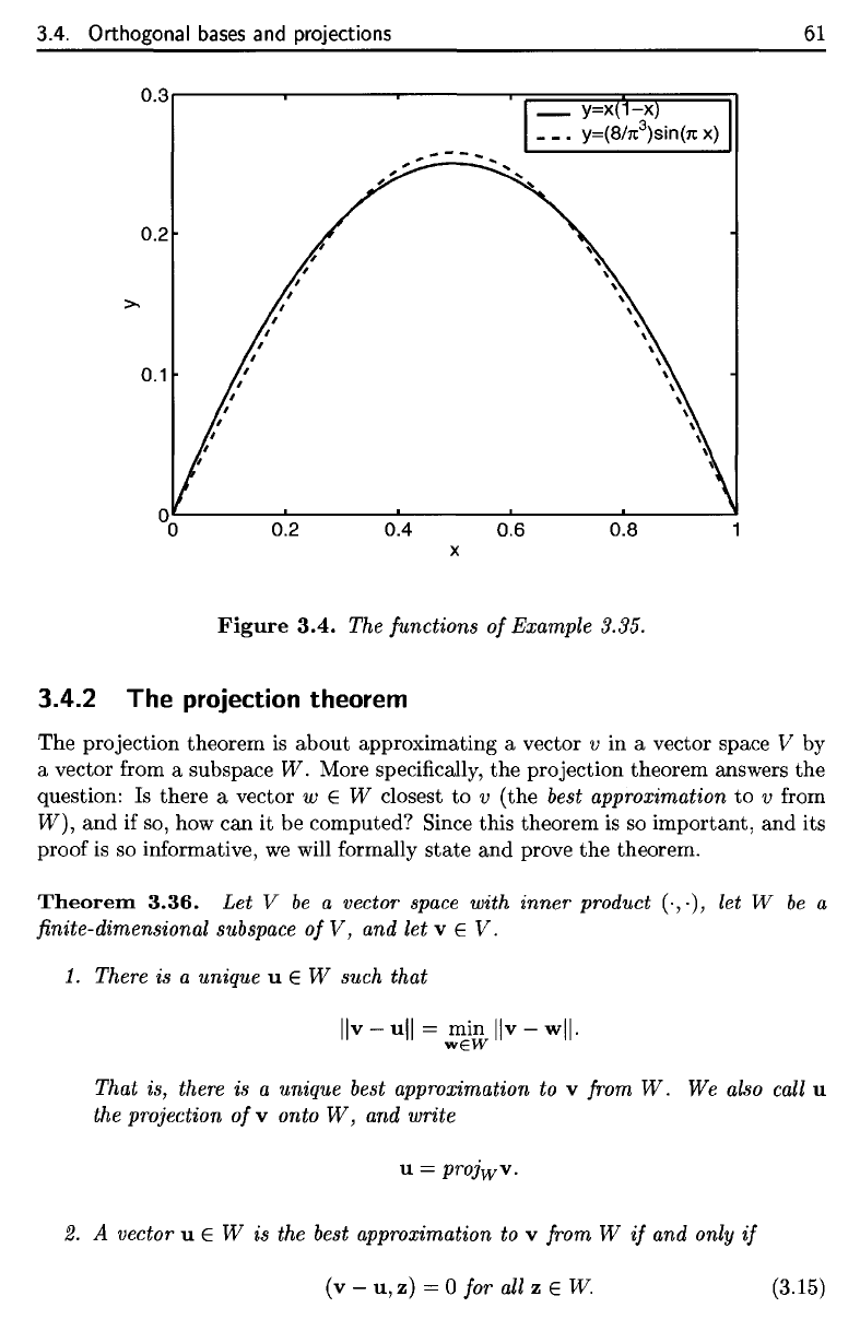
Figure

3.4.

The

functions

of

Example 3.35.

3.4.2

The

projection

theorem

The

projection theorem

is

about

approximating

a

vector

v in a

vector space

V by

a

vector

from

a

subspace

W.

More specifically,

the

projection theorem answers

the

question:

Is

there

a

vector

w

£ W

closest

to v

(the

best

approximation

to v

from

W),

and if so, how can it be

computed? Since this theorem

is so

important,

and its

proof

is so

informative,

we

will

formally

state

and

prove

the

theorem.

Theorem

3.36.

Let V be a

vector

space

with inner product

(-,-),

let W be a

finite-dimensional

subspace

ofV,

and

letv^V.

1.

There

is a

unique

u G W

such that

That

is,

there

is a

unique

best

approximation

to v

from

W.

We

also

call

u

the

projection

o/v

onto

W,

and

write

2. A

vector

u E W is the

best

approximation

to v

from

W if and

only

if

3.4. Orthogonal

bases

and

projections

61

0.3r-------..---~---_r_;::=:::::::::;::3r:=;;===iI

.......

--

.......

0.1

0.2

0.4

0.6

0.8

x

Figure

3.4.

The functions

of

Example 3.35.

3.4.2

The

projection theorem

The

projection theorem

is

about

approximating a vector v in a vector space V by

a vector from a subspace

W.

More specifically,

the

projection theorem answers the

question: Is there a vector

w E W closest

to

v (the best approximation

to

v from

W),

and

if so, how can it be computed? Since this theorem is so important, and its

proof is so informative,

we

will formally

state

and

prove

the

theorem.

Theorem

3.36.

Let V

be

a vector space with inner product (', .), let W

be

a

finite-dimensional subspace

of

V,

and let v E

V.

1.

There is a unique u E W such that

Ilv

- ull = min

Ilv

- wll·

wEW

That is, there is a unique best approximation to v from

W.

We also call u

the projection

of

v onto

W,

and write

u =

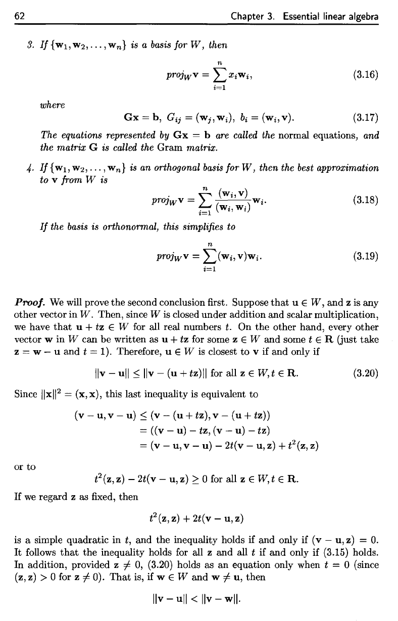
projwv.

2.

A vector u E W is the best approximation to v from W

if

and only

if

(v -

u,

z) = 0 for all z E

W.

(3.15)

62

Chapter

3.

Essential

linear

algebra

3.

If

{wi,

w

2

,...,

w

n

}

is a

basis

for

W,

then

where

The

equations

represented

by Gx = b are

called

the

normal

equations,

and

the

matrix

G is

called

the

Gram matrix.

4-

If

(w

1;

w

2

,...,

w

n

}

is an

orthogonal

basis

for

W,

then

the

best

approximation

to

v

from

W is

If

the

basis

is

orthonormal,

this

simplifies

to

Proof.

We

will

prove

the

second conclusion

first.

Suppose

that

u

e

W,

and z is any

other vector

in

W.

Then, since

W is

closed under addition

and

scalar

multiplication,

we

have

that

u + tz € W for all

real numbers

t. On the

other hand, every other

vector

w in W can be

written

as u + tz for

some

z £ W and

some

t € R

(just

take

z

—

w

—

u and t =

1).

Therefore,

u € W is

closest

to v if and

only

if

If

we

regard

z as fixed,

then

or

to

is

a

simple quadratic

in t, and the

inequality holds

if and

only

if (v - u, z) = 0.

It

follows

that

the

inequality holds

for all z and all t if and

only

if

(3.15) holds.

In

addition, provided

z

/

0,

(3.20) holds

as an

equation only when

t = 0

(since

(z,

z) > 0 for z

^

0).

That

is, if w € W and w

^

u,

then

Since

||x||

2

=

(x,x),

this

last

inequality

is

equivalent

to

62

Chapter

3.

Essential linear algebra

3.

If

{WI,

W2,

...

, w

n

}

is a basis for

W,

then

where

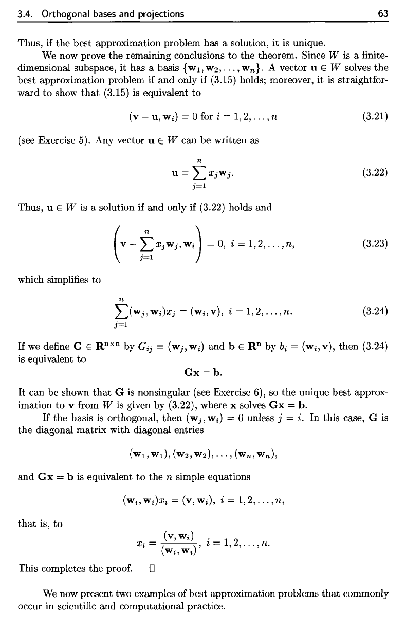
n

projw

v

=

LXiWi,

i=1

(3.16)

Gx

=

b,

G

ij

=

(Wj,

Wi),

b

i

=

(Wi,

v). (3.17)

The equations represented

by

Gx

= b

are

called the normal equations, and

the matrix

G is called the Gram matrix.

4·

If

{Wl,

W2,···,

w

n

}

is an orthogonal basis for W, then the best approximation

to

v from W is

.

~

(Wi'V)

proJw

v

=

~

( . .)Wi.

i=1

W"

W,

If

the basis is orthonormal, this simplifies to

n

projw

v

=

L(Wi,

V)Wi.

i=l

(3.18)

(3.19)

Proof.

We

will prove the second conclusion first. Suppose

that

u E

W,

and z

is

any

other vector in

W.

Then, since W

is

closed under addition and scalar multiplication,

we

have

that

u +

tz

E W for all real numbers t. On

the

other hand, every other

vector

W in W can be written as u +

tz

for some z E W and some t E R (just take

z

= W - u and t = 1). Therefore, u E W

is

closest to v if and only

if

Ilv

-

ull

s:

IIv

-

(u

+

tz)11

for all z E

W,

t E

R.

Since

IIxl1

2

=

(x,x),

this last inequality is equivalent to

or

to

(v -

u,

v - u)

s:

(v -

(u

+

tz),

v -

(u

+ tz))

= ((v - u) - tz, (v - u) - tz)

= (v -

u,

v - u) - 2t(v -

u,z)

+

e(z,z)

t

2

(z,

z) - 2t(v -

u,

z)

2':

0 for all z E

W,

t E

R.

If

we

regard z as fixed, then

e(z,z)+2t(v-u,z)

(3.20)

is a simple quadratic in

t, and the inequality holds if and only if (v -

u,

z) =

O.

It

follows

that

the inequality holds for all z and all t if

and

only if (3.15) holds.

In addition, provided z

i-

0,

(3.20) holds as an equation only when t = 0 (since

(z, z) > 0 for z

i-

0).

That

is, if W E W and W

i-

u,

then

IIv-ull < IIv-wlI·

3.4. Orthogonal

bases

and

projections

63

Thus,

if the

best

approximation problem

has a

solution,

it is

unique.

We

now

prove

the

remaining conclusions

to the

theorem. Since

W is a finite-

dimensional subspace,

it has a

basis

{wi,

w

2

,...,

w

n

}.

A

vector

u

e

W

solves

the

best approximation problem

if and

only

if

(3.15) holds; moreover,

it is

straightfor-

ward

to

show

that

(3.15)

is

equivalent

to

(see

Exercise

5).

Any

vector

u G W can be

written

as

Thus,

u 6 W is a

solution

if and

only

if

(3.22)

holds

and

which

simplifies

to

If

we

define

G 6

R

nxn

by

Gy

=

(w

j?

Wj)

and b 6

R

n

by

b

t

=

(w

i?

v),

then

(3.24)

is

equivalent

to

It can be

shown

that

G is

nonsingular (see Exercise

6),

so the

unique

best

approx-

imation

to v

from

W is

given

by

(3.22),

where

x

solves

Gx = b.

If

the

basis

is

orthogonal,

then

(wj,

w;)

= 0

unless

j = i. In

this

case,

G is

the

diagonal matrix with diagonal entries

and Gx

—

b is

equivalent

to the

n

simple equations

that

is, to

This completes

the

proof.

We

now

present

two

examples

of

best approximation problems

that

commonly

occur

in

scientific

and

computational practice.

3.4. Orthogonal bases and projections 63

Thus, if

the

best approximation problem has a solution,

it

is unique.

We

now prove

the

remaining conclusions

to

the

theorem. Since W is a finite-

dimensional subspace,

it

has a basis

{WI,

W2,

...

, w

n

}.

A vector u E W solves

the

best approximation problem if and only if (3.15) holds; moreover,

it

is

straightfor-

ward

to

show

that

(3.15) is equivalent

to

(v

-

u,

Wi)

= 0 for i = 1,2,

...

, n

(see Exercise 5). Any vector u E W can be written as

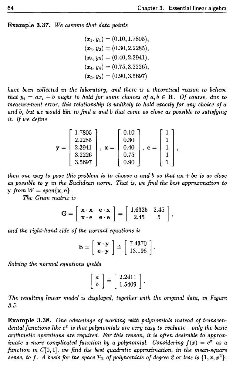
n

u=

LXjWj.

j=1

Thus, u E W

is

a solution if and only if (3.22) holds

and

which simplifies

to

(

V -

"tXjWj,

Wi) = 0, i = 1,2,

...

,n,

)=1

n

L(Wj,Wi)Xj

= (Wi,V), i =

1,2,

...

,n.

j=1

(3.21)

(3.22)

(3.23)

(3.24)

If

we

define G E R

nxn

by G

ij

=

(Wj,

Wi)

and

bERn

by b

i

=

(Wi,

v), then (3.24)

is equivalent

to

Gx=b.

It

can be shown

that

G is nonsingular (see Exercise 6), so

the

unique best approx-

imation

to

v from W is given by (3.22), where x solves

Gx

=

b.

If

the basis is orthogonal,

then

(Wj,

Wi)

= 0 unless j = i. In this case, G is

the

diagonal matrix with diagonal entries

and

Gx

= b

is

equivalent

to

the

n simple equations

that

is,

to

(v,

Wi)

Xi

= )' i = 1,2,

...

,n.

(Wi,Wi

This completes

the

proof. 0

We

now present two examples of best approximation problems

that

commonly

occur in scientific

and

computational practice.

64

Chapter

3.

Essential

linear

algebra

Example

3.37.

We

assume that data points

(xi,yi)

=

(0.10,1.7805),

(z

2

,!fe)

=

(0.30,2.2285),

(z

3

,2/

3

)

=

(0.40,2.3941),

(0:4,2/4)

=

(0.75,3.2226),

(a*,2/5)

-(0.90,3.5697)

have

been collected

in the

laboratory,

and

there

is a

theoretical reason

to

believe

that

yi

=

axi

+ b

ought

to

hold

for

some choices

of

a, b 6 R. Of

course,

due to

measurement error, this relationship

is

unlikely

to

hold exactly

for any

choice

of

a

and b, but we

would like

to find a and b

that come

as

close

as

possible

to

satisfying

it. If we

define

then

one way to

pose this problem

is to

choose

a and b so

that

ax + be is as

close

as

possible

to y in the

Euclidean

norm.

That

is, we find the

best approximation

to

y

from

W =

span{x,

e).

The

Gram

matrix

is

The

resulting linear model

is

displayed,

together with

the

original data,

in

Figure

3.5.

Example

3.38.

One

advantage

of

working with polynomials instead

of

transcen-

dental

functions like

e

x

is

that polynomials

are

very easy

to

evaluate—only

the

basic

arithmetic operations

are

required.

For

this reason,

it is

often

desirable

to

approx-

imate

a

more complicated

function

by a

polynomial. Considering

f(x]

=

e

x

as a

function

in

(7[0,1],

we find the

best quadratic approximation,

in the

mean-square

sense,

to

f.

A

basis

for the

space

V^

of

polynomials

of

degree

2 or

less

is

{l,x,x

2

}.

and

the

right-hand side

of the

normal equations

is

Solving

the

normal equations yields

64

Chapter 3. Essential linear algebra

Example

3.37.

We assume that data points

(xl,yd

= (0.10,1.7805),

(X2,

Y2)

= (0.30,2.2285),

(X3,

Y3)

= (0.40,2.3941),

(X4,

Y4)

= (0.75,3.2226),

(X5,Y5) = (0.90,3.5697)

have

been

collected in the laboratory, and there is a theoretical reason to believe

that

Yi

= aXi + b ought to hold for some choices

of

a, b E

R.

Of

course, due to

measurement error, this relationship is unlikely to hold exactly for any choice

of

a

and

b,

but

we

would like to find a and b that come

as

close

as

possible to satisfying

it.

If

we

define

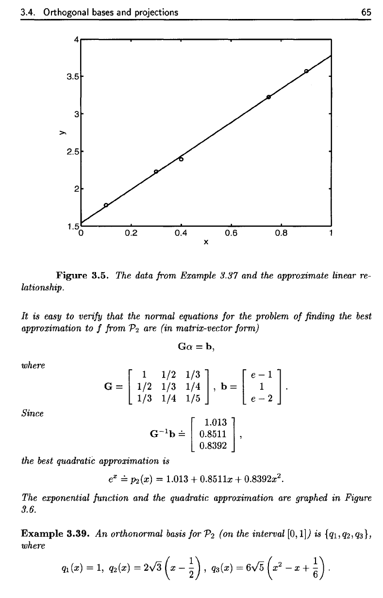
Y=[H~:~

,x~

3.2226

3.5697

0.10

I

0.30

0.40

,e

=

0.75

0.90

1

then one way to pose this problem is to choose a and b

so

that

ax

+ be is

as

close

as

possible to y

in

the Euclidean norm. That is,

we

find the best approximation to

y from W = span{x, e}.

The Gram matrix is

G = [

x·

x

e·

x ] =

[1.6325

2.45]

x . e

e·

e

2.45

5 '

and the right-hand side

of

the normal equations is

b = [

x·

y ]

==

[ 7.4370 ]

e·

y

13.196·

Solving the normal equations yields

[

a]

==

[ 2.2411 ]

b

1.5409'

The resulting linear model is displayed, together with the original data,

in

Figure

3.5.

Example

3.38.

One advantage

of

working with polynomials instead

of

transcen-

dental functions like

eX

is that polynomials

are

very easy to

evaluate~only

the basic

arithmetic operations

are

required. For this reason,

it

is often desirable to approx-

imate a more complicated function by a polynomial. Considering

f(x)

=

eX

as

a

function

in

C(O,

1],

we

find the best quadratic approximation,

in

the mean-square

sense, to

f.

A basis for the space

P2

of

polynomials

of

degree

2 or less is

{I,

x,

x

2

}.

3.4.

Orthogonal

bases

and

projections

65

Figure

3.5.

The

data from Example 3.37

and the

approximate linear

re-

lationship.

It is

easy

to

verify

that

the

normal equations

for the

problem

of finding the

best

approximation

to f

from

p2 are (in

matrix-vector form)

where

Since

the

best quadratic approximation

is

The

exponential

function

and the

quadratic approximation

are

graphed

in

Figure

3.6.

Example

3.39.

An

orthonormal basis

for

p2 (on the

interval

[0,1]J

is

{^1,^25^3};

where

Ga

= b,

3.4. Orthogonal bases and projections

65

4~------~------~------~~------~------~

x

Figure

3.5.

The data from Example 3.37 and the approximate linear

re-

lationship.

It

is easy to verify that the normal equations for the problem

of

finding the best

approximation to f from

P2

are

(in matrix-vector form)

where

Since

G = [

1~2

1/3

1/2

1/3

1/4

Ga=b,

1/3

] [ e - 1 ]

1/4

,b

= 1 .

1/5 e - 2

G-1b

==

0.8511 ,

[

1.013]

0.8392

the best quadratic approximation is

eX

==

JJ2{x)

= 1.013 + 0.8511x + 0.8392x2.

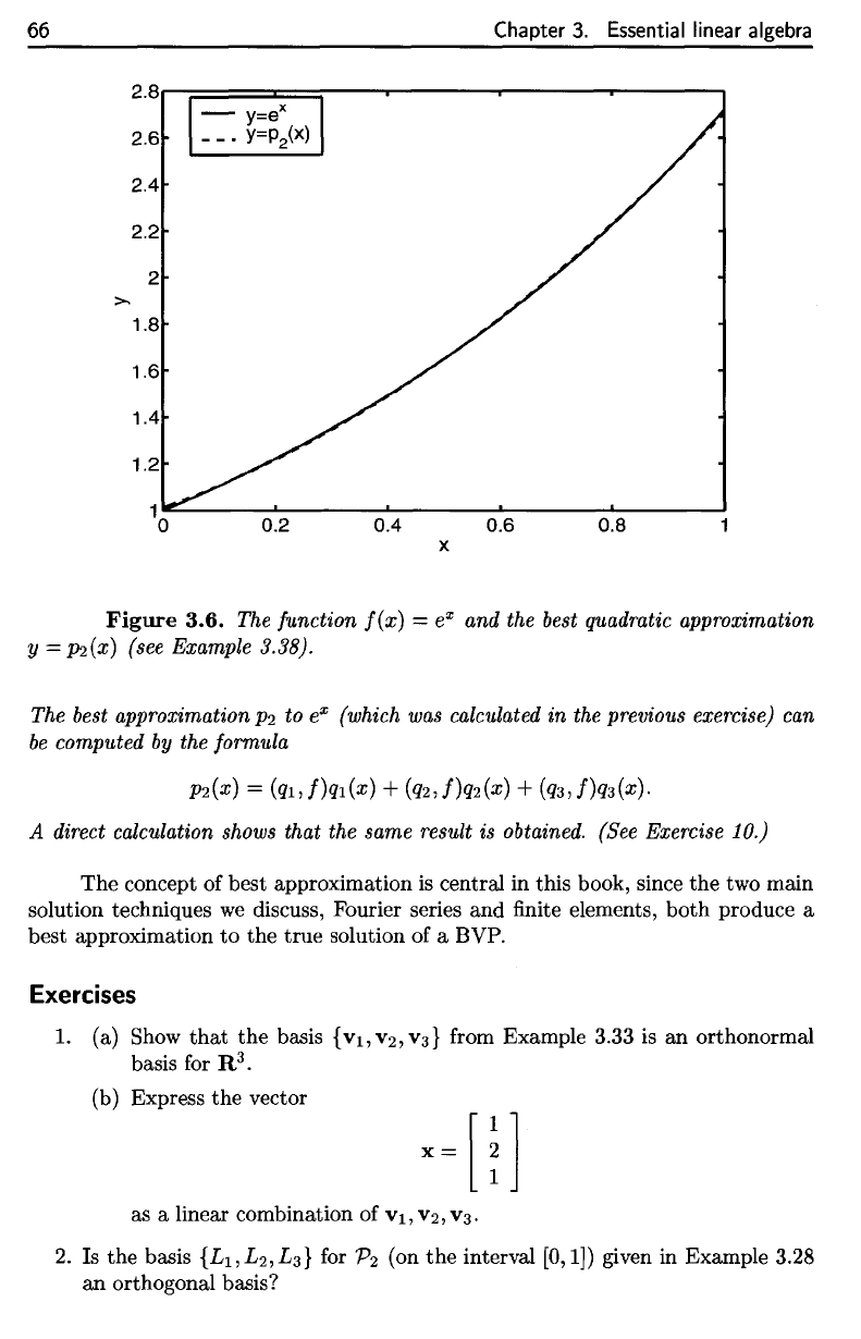
The exponential function and the quadratic approximation

are

graphed

in

Figure

3.6.

Example

3.39.

An

orthonormal basis for P

2

(on the interval [0,1]) is {ql, Q2,

Q3},

where

66

Chapter

3.

Essential linear algebra

Figure

3.6.

The

function

f(x)

—

e

x

and the

best

quadratic

approximation

y

—

Pi(x)

(see Example 3.38).

Exercises

1. (a)

Show

that

the

basis

{vi,v

2

,V3}

from

Example 3.33

is an

orthonormal

basis

for R

3

.

(b)

Express

the

vector

as a

linear combination

of

YI

,

V2,

\s.

2.

Is the

basis

{1/1,1/2,1/3}

for

P

2

(on the

interval

[0,1])

given

in

Example 3.28

an

orthogonal basis?

The

concept

of

best approximation

is

central

in

this book, since

the two

main

solution techniques

we

discuss, Fourier series

and finite

elements, both produce

a

best

approximation

to the

true solution

of a

BVP.

A

direct

calculation shows that

the

same result

is

obtained. (See Exercise 10.)

P2(x)

=

(qij)qi(x)

+

(q2,f}qi(x)

+

(tfs,/)^).

The

best

approximation

p^

to

e

x

(which

was

calculated

in the

can

be

computed

by the

formula

66

Chapter

3.

Essential linear algebra

2.8

2.6

-

y=e

x

-

_.

y=P2(X)

2.4

2.2

2

>-

1.8

1.6

1.4

1.2

1

0 0.2 0.4 0.6 0.8

x

Figure

3.6.

The function

f(x)

=

eX

and the best quadratic approximation

y =

p2(X)

(see Example 3.38).

The best approximation

P2

to

eX

(which was calculated in the previous exercise) can

be

computed

by

the formula

A direct calculation shows that the same result is obtained. (See Exercise 10.)

The

concept of best approximation

is

central in this book, since the two main

solution techniques

we

discuss, Fourier series and finite elements,

both

produce a

best approximation

to

the

true

solution of a BVP.

Exercises

1.

(a) Show

that

the

basis

{VI,

V2,

V3}

from Example 3.33

is

an orthonormal

basis for R

3

.

(b) Express the vector

as a linear combination of

VI,

V2, V3.

2.

Is the basis {L

I

,L

2

,L

3

}

for

P2

(on

the

interval [0,1]) given in Example 3.28

an

orthogonal basis?

3.4. Orthogonal

bases

and

projections

67

if

and

only

if (x, y) = 0.

4.

Use the

results

of

this

section

to

show

that

any

orthonormal

set

containing

n

vectors

in

R

n

is a

basis

for

R

n

.

(Hint: Since

the

dimension

of

R

n

is n, it

suffices

to

show either

that

the

orthogonal

set

spans

R

n

or

that

it is

linearly

independent. Linear independence

is

probably easier.)

5.

Let W be a

subspace

of an

inner product space

V and let

{wi,

w

2

,...,

w

n

}

be

a

basis

for

W.

Show

that,

for y

e

V,

holds

if and

only

if

holds.

6.

Let

{w

1;

w

2

,...,

w

n

}

be a

linearly independent

set in an

inner product space

y, and

define

G

e

R

nxn

by

X

1.0000

1.2500

1.4000

1.5000

1.9000

2.1000

2.2500

2.6000

2.9000

y

2.0087

2.4907

2.8363

2.9706

3.9092

4.1932

4.5057

5.2533

5.8030

3.

Let V be an

inner product space. Prove

that

x, y

e

V

satisfy

Prove

that

G is

invertible. Hint:

By the

Fredholm

alternative,

it

suffices

to

show

that

the

only solution

to Gx

=

0 is x = 0.

Assume

that

x E

R

n

satisfies

Gx = 0.

This implies

that

Show

that

x • Gx

=

(u,

u),

where

u

€ V is

given

by

and

show

that

u

cannot

be the

zero vector unless

x = 0.

7.

Consider

the

following

data:

(y, z) = 0 for all z G W

Gij

=

(wj-jWj),

i,j

=

1,2,...,n.

3.4. Orthogonal bases and projections

67

3.

Let V be

an

inner product space. Prove

that

x, y E V satisfy

if and only if (x,

y) =

O.

4.

Use the results of this section

to

show

that

any orthonormal set containing

n vectors in R n

is

a basis for R

n.

(Hint: Since the dimension of R n

is

n,

it

suffices

to

show either

that

the orthogonal set spans Rn or

that

it

is

linearly

independent. Linear independence

is

probably easier.)

5.

Let W be a subspace of

an

inner product space V and let {Wi,

W2,

...

, w

n

}

be a basis for W. Show

that,

for y E V,

(y, z) = 0 for all z E W

holds if and only if

(y,Wi)

=0,

i=1,2,

...

,n

holds.

6.

Let {Wi,

W2,

...

, w

n

}

be

a linearly independent set in

an

inner product space

V, and define G E R

nxn

by

G

ij

=

(Wj,Wi),

i,j

= 1,2,

...

,n.

Prove

that

G

is

invertible. Hint: By the Fredholm alternative, it suffices

to

show

that

the

only solution

to

Gx

= 0

is

x =

O.

Assume

that

x E Rn satisfies

Gx

=

O.

This implies

that

x·Gx

=

O.

Show

that

X·

Gx

= (u, u), where u E V

is

given by

and show

that

u cannot be

the

zero vector unless x =

o.

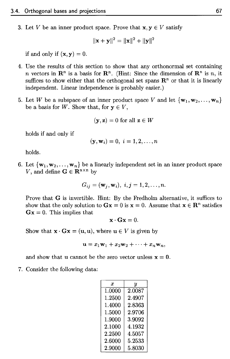
7.

Consider the following data:

x

y

1.0000 2.0087

1.2500 2.4907

1.4000 2.8363

1.5000 2.9706

1.9000 3.9092

2.1000 4.1932

2.2500 4.5057

2.6000

5.2533

2.9000 5.8030

Gockenbach M.S. Partial Differential Equations. Analytical and Numerical Methods

Подождите немного. Документ загружается.