Gockenbach M.S. Partial Differential Equations. Analytical and Numerical Methods
Подождите немного. Документ загружается.

38
Chapter
3.
Essential linear algebra
8.
(a)
Suppose
/ : R
2
—>•
R
2
is
linear. Prove
that
there
is a
matrix
A €
R
2x2
such
that
/ is
given
by
/(x)
= Ax.
Hint: Each
x
e
R
2
satisfies
x =
xiei
+
#262,
where
Since
/ is
linear,
we
have
The
desired matrix
A can be
expressed
in
terms
of the
vectors
/(ei),
/(e
2
).
(b)
Now
show
that
if / :
R
n
—>•
R
m
is
linear, then there exists
a
matrix
A
<E
R
mxn
such
that
/(x)
= Ax for all x e
R
n
.
3.2
Existence
and
uniqueness
of
solutions
to Ax = b
We
will
now
discuss
the
linear system
Ax = b,
where
A e
R
nxn
and b e
R
n
,
as a
linear
operator
equation.
We
consider three fundamental questions:
1.
Does
a
solution
to the
equation exist?
2.
If a
solution exists,
is it
unique?
3. If a
unique solution exists,
how can we
compute
it?
It
turns
out
that
the first two
questions
are
intimately linked;
the
purpose
of
this
section
is to
shed some light
on
these
two
questions
and the
connection between
them.
We
will
also
briefly
discuss
how
this point
of
view
can be
carried over
to the
case
of a
linear
differential
equation.
The
third question
will
be
deferred
to
later
in
this chapter.
3.2.1 Existence
The
existence
of a
solution
to Ax = b is
equivalent
to the
condition
that
b lie in
72-(A),
the
range
of A.
This begs
the
question:
What
sort
of a set is
7£(A)?
If
y, w 6
72.(A),
say y = Ax, w = Az,
then
This
shows
that
ay +
/3w
€
72-(A).
Moreover,
the
zero vector lies
in
7£(A),
since
AO
= 0. It
follows
that
7£(A)
is a
subspace
of
R
n
(possibly
the
entire space
R
n
—
every
vector space
is a
subspace
of
itself).
Every linear operator
has
this property;
if
f : X
-»
Y is a
linear operator, then
72-(f)
is a
subspace
of the
vector space
Y.
(The same need
not be
true
for a
nonlinear operator.)
38
Chapter
3.
Essential
linear
algebra
8. (a) Suppose f : R2
-t
R2
is
linear. Prove
that
there
is
a matrix A E R
2X2
such
that
f
is
given by
f(x)
=
Ax.
Hint: Each x E R2 satisfies x =
Xlel +X2e2, where
Since
f
is
linear,
we
have
The
desired matrix A can be expressed in terms of the vectors f
(et),
f(e2).
(b)
Now
show
that
if
f : R
II
-t
R m
is
linear, then there exists a matrix
A E
RmXll such
that
f(x)
=
Ax
for all x E
Rll.
3.2
Existence and uniqueness
of
solutions
to
Ax
= b
We
will now discuss
the
linear system
Ax
=
b,
where A E RllXll and b E
Rll,
as a
linear operator equation.
We
consider three fundamental questions:
1. Does a solution to the equation exist?
2.
If
a solution exists,
is
it
unique?
3.
If
a unique solution exists, how can
we
compute it?
It
turn~
out
that
the
first two questions are intimately linked;
the
purpose of this
section
is
to shed some light on these two questions and the connection between
them.
We
will also briefly discuss how this point of view can be carried over to
the
case of a linear differential equation.
The
third
question will be deferred
to
later in
this chapter.
3.2.1 Existence
The
existence of a solution to
Ax
= b
is
equivalent
to
the
condition
that
b lie in
R(A),
the range of
A.
This begs
the
question:
What
sort of a set
is
R(A)?
If
y,
wE
R(A),
say y =
Ax,
w =
Az,
then
ay
+
{3w
=
aAx
+
{3Az
=
A(ax
+
(3z).
This shows
that
ay
+
(3w
E
R(A).
Moreover,
the
zero vector lies in
R(A),
since
AO
=
o.
It
follows
that
R(A)
is
a subspace of
Rll
(possibly
the
entire space
Rll-
every vector space
is
a subspace of itself). Every linear operator has this property;
if f : X
-t
Y
is
a linear operator, then
R(f)
is
a subspace of
the
vector space Y.
(The same need not be
true
for a nonlinear operator.)
3.2. Existence
and
uniqueness
of
solutions
to Ax = b 39
The
geometry
of
subspaces
of
R
n
is
particularly simple:
the
proper
subspaces
of
R
n
(i.e. those
that
are not the
entire space)
are
lower-dimensional spaces: lines
in
R
2
,
lines
and
planes
in R
3
, and so
forth
(we
cannot visualize
these
objects
in
dimensions
greater
than
three,
but we can
understand them
by
analogy). Since
every
subspace must contain
the
zero vector,
not
every line
in
R
2
,
for
example,
is
a
subspace,
but
only those passing through
the
origin are.
With this understanding
of the
geometry
of
R
n
,
we
obtain
the
following
con-
clusions:
If
7£(A)
=
R
n
,
then
Ax = b has a
solution
for
each
b
e
R
n
.
(This
is a
tautology.)
If
7£(A)
^
R
n
,
then
Ax = b
fails
to
have
a
solution
for
almost every
b e
R
n
.
This
is
because
a
lower-dimensional subspace comprises very
little
of
R
n
(think
of
a
line contained
in the
plane
or in
three-dimensional
space).
Example
3.13.
We
consider
the
equation
Ax =
b,
where
A 6
R
2x2
is
given
by
For
any x 6
R
2
,
we
have
This
calculation shows that
every
vector
b in the
range
of A is a
multiple
of the
vector
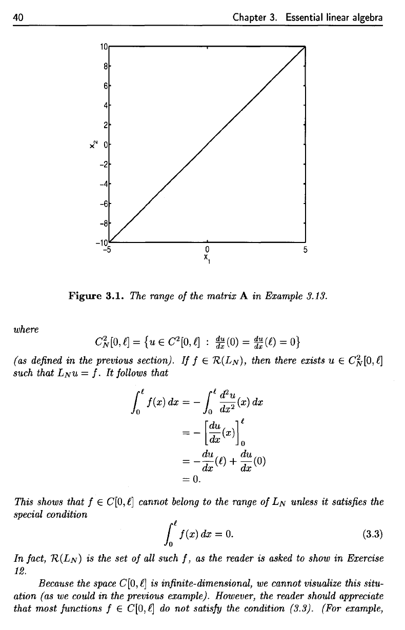
Therefore,
the
subspace
'R-(A)
is a
line
in the
plane
R
2
(see Figure 3.1). Since this
line
is a
very
small part
of
R
2
,
the
system
Ax = b
fails
to
have
a
solution
for
almost
every
b e
R
2
.
As
mentioned
at the
beginning
of
this
chapter, there
is a
close analogy between
linear (algebraic) systems
and
linear differential equations.
The
reader should think
carefully
about
the
similarities between
the
following
example
and the
previous one.
Example
3.14.
We
define
the
linear
differential
operator
LN
'•
C^[Q,f\
-»
(7[0,£j
by
3.2. Existence
and
uniqueness
of
solutions
to
Ax
= b
39
The geometry
of
subspaces of
Rll
is
particularly simple:
the
proper subspaces
of R
II
(Le.
those
that
are not the entire space) are lower-dimensional spaces: lines
in R2, lines and planes in R
3
, and so forth
(we
cannot visualize these objects in
dimensions greater
than
three,
but
we
can understand them by analogy). Since
every subspace must contain the zero vector, not every line in R
2
,
for example,
is
a subspace,
but
only those passing through the origin are.
With
this understanding of the geometry of Rll,
we
obtain
the
following con-
clusions:
•
If
R(A)
= Rll,
then
Ax
= b has a solution for each b E Rll. (This
is
a
tautology. )
•
If
R(A)
i- Rll, then
Ax
= b fails
to
have a solution for almost every b E Rll.
This
is
because a lower-dimensional subspace comprises very little of R
II
(think
of a line contained in
the
plane or in three-dimensional space).
Example
3.13.
We consider the equation
Ax
=
b,
where A E R
2X2
is given
by
A=[~
~].
For any x E R2,
we
have
[
Xl
+
2X2
-
2Xl
+
4X2
=
(Xl
+
2X2)
[
~
] .
This calculation shows that every vector b in the range
of
A is a multiple
of
the
vector
Therefore, the subspace
R(A)
is a line
in
the plane R2 (see Figure 3.1). Since this
line is a very small part
of
R
2
,
the system
Ax
= b fails to have a solution for
almost every
bE
R2.
As
mentioned
at
the
beginning of this chapter, there
is
a close analogy between
linear (algebraic) systems and linear differential equations.
The
reader should think
carefully
about
the similarities between the following example and the previous one.
Example
3.14.
We define the linear differential operator
LN
:
e1[o,
£]
-+
e[O,
£]
by
40
Chapter
3.
Essential linear algebra
Figure
3.1.
The
range
of
the
matrix
A in
Example 3.13.
where
In
fact,
7£(Ljv)
i-
s
the
set of all
such
f,
as the
reader
is
asked
to
show
in
Exercise
12.
Because
the
space
C[0,^]
is
infinite-dimensional,
we
cannot visualize this
situ-
ation
(as we
could
in the
previous example). However,
the
reader
should
appreciate
that most functions
f
e
C[0,
£]
do not
satisfy
the
condition (3.3). (For example,
This
shows that
f
e
C[0,^]
cannot
belong
to the
range
of
LN
unless
it
satisfies
the
special
condition
(as
defined
in the
previous section).
If
f
e
7£(Ljv),
then
there exists
u €
C^[0,l]
such that
LNU
= f. It
follows that
40
Chapter
3.
Essential
linear
algebra
Figure
3.1.
The range
of
the matrix A
in
Example 3.13.
where
CMO,l] =
{u
E C
2
[0,l] :
~~(O)
=
~~(l)
=
O}
(as defined
in
the previous section).
If
f E
R(L
N
), then there exists u E Ch[O,l]
such that
LNu
=
f.
It
follows that
r
l
rl
cPu
io
f(x)
dx
= -
io
dx
2
(x)
dx
[
dU
]1
= -
-(x)
dx 0
= _ du (l) + du
(0)
dx dx
=
0.
This shows that f E
C[O,
l]
cannot belong to the range
of
LN
unless
it
satisfies the
special condition
11
f(x)
dx =
0.
(3.3)
In
fact,
R(LN)
is the set
of
all such
f,
as
the reader is asked to show
in
Exercise
12.
Because the space
C[O,
l]
is infinite-dimensional,
we
cannot visualize this situ-
ation (as
we
could
in
the previous example). However, the reader should appreciate
that
most
functions f E
e[O,
l]
do
not
satisfy the condition (3.3). (For example,
3.2. Existence
and
uniqueness
of
solutions
to Ax = b 41
the
reader
is
invited
to
write down
a
quadratic polynomial
at
random
and
call
it
/(#).
Chances
are
that this quadratic
will
not
satisfy
(3.3).)
Therefore,
the
range
of
LN
is
only
a
small part
of
C[0,i],
and for
most choices
of f
G
C[0,
£],
there
is
no
solution
to
L^u
=
f.
Example
3.15.
We now
define
L
D
:
C^[Q,l]
->•
C[Q,f\
by
where
The
reader
should
recall
from
the
previous section that
the
BVP
can be
written
as the
linear
operator
equation
Lj^u
—
f.
We
will
show that
'R-(A)
is
all
of
C[Q,(]
by
showing that
we can
solve
Lpu
= f for
every
f £
C[0,£].
The
idea
is
to
integrate twice
and use the
boundary
conditions
to
determine
the
constants
of
intearation.
We
have
so
We
write
where
We
then
integrate
to
obtain
The
reader
should notice
the use of the
dummy variables
of
integration
s and z.
The
first
boundary
condition,
w(0)
=
0,
implies that
Ci
= 0. We
then have
since
u(i]
—
0,
we
obtain
3.2.
Existence
and
uniqueness
of
solutions
to
Ax
= b
41
the reader is invited
to
write
down
a quadratic polynomial at random and
call
it
f(x).
Chances
are
that this quadratic will not satisfy (3.3).) Therefore, the
range
of LN
is
only a small part of
C[O,
f],
and for most choices
of
f E
C[O,
f],
there
is
no
solution
to
LNU
=
f.
Example
3.15.
We
now define
LD
: Cb[O,f]-+
C[O,f]
by
d
2
u
LDU
= - dx
2
'
where
Cb[O,f] =
{u
E C2[0,f] :
u(O)
= u(f) =
O}.
The
reader should
recall
from the previous section that the B VP
~u
- dx
2
=
f(x),
° < x <
f,
u(O)
= 0,
u(f) = °
can
be
written
as
the linear operator equation L
DU
= f .
We
will
show
that R(
A)
is
all
of
C[O,
f]
by
showing that
we
can
solve
LDu = f for every f E
C[O,
fl.
The
idea
is
to
integrate twice and use the boundary conditions
to
determine the constants
of
integration.
We
have
~U
dx
2
(x) =
-f(x),
° < x <
f,
so
du
l
X
dx (x) = - 0 f(s)
ds
+ C
b
a < x <
f.
We
write
du
dx(X) =
-F(x)
+c
1 , ° < x < f,
where
F(x) =
fox
f(s) ds.
We
then integrate
to
obtain
u(x)
=
-loX
F(z)
dz + C
1
x + C
2
=
-loX
Io
z
f(s)
dsdz
+ C
1
x + C
2
, ° < X <
f.
The
reader should notice the use of the dummy variables of integration
sand
z.
The
first boundary condition,
u(O)
=
0,
implies that C
2
=
O.
We
then have
u(f)
=
-10£
l
z
f(s)
dsdz
+ C
1
f;
since u(f) = 0,
we
obtain
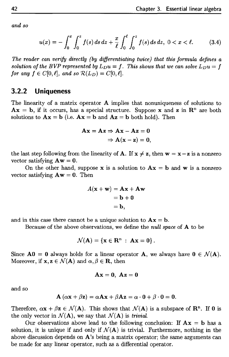
1111Z
C
1
= e 0 0
f(s)dsdz
42
Chapter
3.
Essential
linear
algebra
and so
The
reader
can
verify
directly
(by
differentiating
twice)
that this formula
defines
a
solution
of
the BVP
represented
by
LDU
=
f.
This
shows
that
we can
solve
LDU
= f
for
any f
e
C[0,4
and so
K(L
D
)
=
C[Q,l}.
3.2.2
Uniqueness
The
linearity
of a
matrix operator
A
implies
that
nonuniqueness
of
solutions
to
Ax = b, if it
occurs,
has a
special structure. Suppose
x and z in
R
n
are
both
solutions
to Ax = b
(i.e.
Ax = b and Az = b
both hold). Then
the
last
step
following
from
the
linearity
of A. If x
^
z,
then
w = x
—
z is a
nonzero
vector
satisfying
Aw = 0.
On
the
other hand, suppose
x is a
solution
to Ax = b and w is a
nonzero
vector
satisfying
Aw = 0.
Then
and
in
this case there cannot
be a
unique solution
to Ax = b.
Because
of the
above observations,
we
define
the
null
space
of A to be
Since
AO
=
0
always holds
for a
linear operator
A, we
always have
0
e
-A/"(A).
Moreover,
if
x,z
e
A/"(A)
and a, ft € R,
then
and so
Therefore,
ax +
/3z
€
A/"(A).
This
shows
that
A/"(A)
is a
subspace
of
R
n
.
If 0 is
the
only vector
in
A/"(A),
we say
that
A/"(A)
is
trivial.
Our
observations above lead
to the
following
conclusion:
If Ax = b has a
solution,
it is
unique
if and
only
if
wV(A)
is
trivial. Furthermore, nothing
in the
above discussion depends
on A's
being
a
matrix operator;
the
same arguments
can
be
made
for any
linear operator, such
as a
differential
operator.
42
Chapter
3.
Essential linear algebra
and so
r r x r
l
r
u(x)=-
1010
f(s)dsdz+
e10
10
f(s)dsdz,
O<x<l.
(3.4)
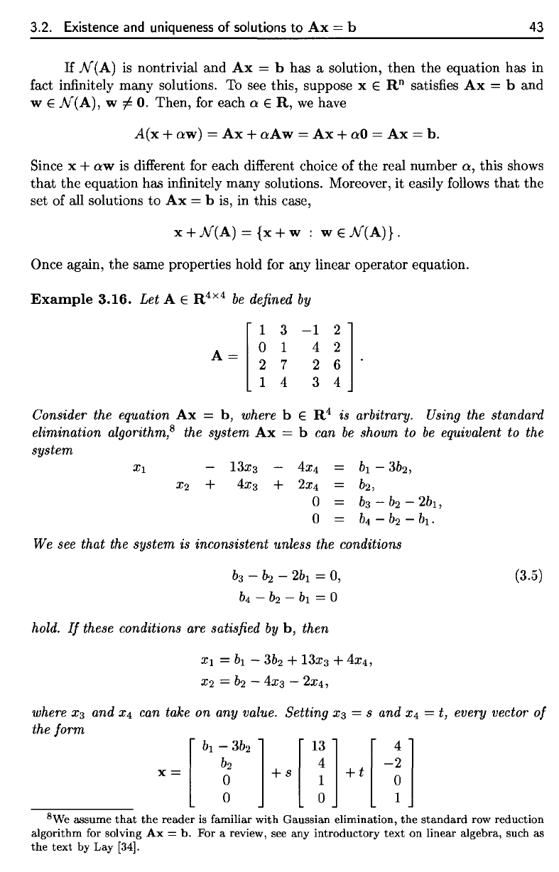
The reader can verify directly (by differentiating twice) that this formula defines a
solution
of
the
BVP
represented by
Lnu
=
f.
This shows that
we
can solve
Ln
u
= f
for any f E C[O,l], and
so
R(Ln)
= C[O,l].
3.2.2 Uniqueness
The linearity of a matrix operator A implies
that
nonuniqueness of solutions
to
Ax
=
b,
if it occurs, has a special structure. Suppose x and z in
Rll
are
both
solutions
to
Ax
= b
(Le.
Ax
=
band
Az
= b both hold). Then
Ax
=
Az
=>
Ax
-
Az
= 0
=>
A(x
- z) = 0,
the last step following from the linearity of
A.
If
x
=I
z, then w = x - z
is
a nonzero
vector satisfying A w
=
o.
On
the
other hand, suppose x
is
a solution
to
Ax
= b and w
is
a nonzero
vector satisfying
Aw
=
o.
Then
A(x+w)
=Ax+Aw
=b+O
=b,
and
in this case there cannot be a unique solution
to
Ax
=
b.
Because of
the
above observations,
we
define the null space of A to be
N(A)
= {x E
Rll
:
Ax
=
O}.
Since
AO
= 0 always holds for a linear operator
A,
we
always have 0 E
N(A).
Moreover, if
x,z
E
N(A)
and
a,{3 E
R,
then
Ax
= 0,
Az
= 0
and
so
A
(ax
+
{3z)
=
aAx
+
{3Az
= a . 0 +
{3
·0=
o.
Therefore,
ax
+
{3z
E
N(A).
This shows
that
N(A)
is
a subspace of
Rll.
If
0
is
the only vector in
N(A),
we
say
that
N(A)
is
trivial.
Our observations above lead
to
the following conclusion:
If
Ax
= b has a
solution,
it
is
unique if and only if
N(A)
is
trivial. Furthermore, nothing in
the
above discussion depends on
A's
being a matrix operator; the same arguments can
be made for any linear operator, such as a differential operator.
3.2. Existence
and
uniqueness
of
solutions
to Ax = b
43
If
JV(A)
is
nontrivial
and Ax = b has a
solution, then
the
equation
has in
fact
infinitely
many solutions.
To see
this, suppose
x
e
R
n
satisfies
Ax = b and
w
e
A/"(A),
w
7^
0.
Then,
for
each
a G R, we
have
8
We
assume
that
the
reader
is
familiar
with Gaussian elimination,
the
standard
row
reduction
algorithm
for
solving
Ax = b. For a
review,
see any
introductory text
on
linear algebra, such
as
the
text
by Lay
[34].
Since
x + aw is
different
for
each
different
choice
of the
real number
a,
this shows
that
the
equation
has
infinitely
many solutions. Moreover,
it
easily
follows
that
the
set
of all
solutions
to Ax = b is, in
this case,
Once
again,
the
same properties hold
for any
linear operator equation.
Example
3.16.
Let A
e
R
4x4
be
defined
by
Consider
the
equation
Ax =
b,
where
b
e
R
4
is
arbitrary.
Using
the
standard
elimination
algorithm,
8
the
system
Ax = b can be
shown
to be
equivalent
to the
system
We
see
that
the
system
is
inconsistent unless
the
conditions
hold.
If
these conditions
are
satisfied
by b.
then
where
x%
and
x±
can
take
on any
value. Setting
#3
= s and
#4
= t,
every
vector
of
the
form
3.2. Existence and uniqueness of solutions
to
Ax
= b
43
If
N(A)
is
nontrivial
and
Ax
= b has a solution,
then
the
equation has in
fact infinitely many solutions. To see this, suppose x E
RD
satisfies
Ax
=
band
wE
N(A),
w
=F
O.
Then, for each
0:
E
R,
we
have
A(x
+ o:w) =
Ax
+ o:Aw =
Ax
+
0:0
=
Ax
=
b.
Since x + o:w is different for each different choice
of
the
real number
0:,
this shows
that
the
equation has infinitely
many
solutions. Moreover,
it
easily follows
that
the
set of all solutions
to
Ax
= b is, in this case,
x+N(A)
=
{x+w
: w
EN(A)}.
Once again,
the
same properties hold for any linear
operator
equation.
Example
3.16.
Let
A E R
4x4
be
defined by
Consider
the equation
Ax
=
b,
where b E
R4
is arbitrary. Using the standard
elimination
algorithm,
8
the
system
Ax
= b can
be
shown
to
be
equivalent to the
system
Xl
13
X
3
4X4
b
l
-
3b
2
,
X2
+
4X3
+
2X4
b
2
,
0
b
3
- b
2
-
2b
l
,
0
b
4
- b
2
- b
l
.
We
see
that
the
system
is
inconsistent
unless the conditions
b
3
-
b
2
-
2b
1
= 0,
b
4
-
b
2
-
b
1
= 0
hold.
If
these conditions are satisfied by
b,
then
Xl
= b
l
-
3b
2
+ 13x3 + 4X4,
X2
= b
2
-
4X3
- 2X4,
(3.5)
where
X3
and
X4
can take
on
any
value.
Setting
X3
=
sand
X4
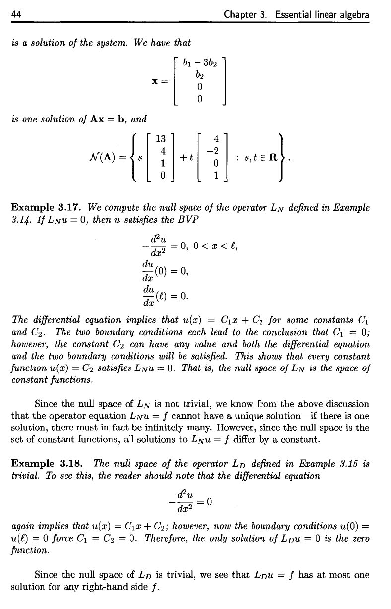
= t, every vector
of
the
form
x=
[
bl
~2
3b
2
] [
1~
] [ -
~
1
o
+s
1
+t
0
001
8We assume
that
the
reader
is familiar
with
Gaussian elimination,
the
standard
row reduction
algorithm
for solving
Ax
=
h.
For
a review, see any
introductory
text
on
linear algebra, such as
the
text
by Lay
[34].
44
Chapter
3.
Essential linear algebra
is a
solution
of the
system.
We
have that
is
one
solution
of
Ax = b, and
Example
3.17.
We
compute
the
null
space
of
the
operator
LN
defined
in
Example
3.14-
If
LNU
=
0,
then
u
satisfies
the BVP
The
differential
equation implies that
u(x]
=
C\x
+
C%
for
some constants
C\
and
C^-
The two
boundary
conditions
each
lead
to the
conclusion that
C\
= 0;
however,
the
constant
C%
can
have
any
value
and
both
the
differential
equation
and
the two
boundary
conditions
will
be
satisfied.
This
shows that
every
constant
function
u(x)
=
C<z
satisfies
LNU = 0.
That
is, the
null
space
of
LN
is the
space
of
constant functions.
Since
the
null space
of
LTV
is not
trivial,
we
know
from
the
above discussion
that
the
operator
equation
L^u
= f
cannot
have
a
unique
solution—if
there
is one
solution, there must
in
fact
be
infinitely many. However, since
the
null space
is the
set of
constant functions,
all
solutions
to
L^u
= f
differ
by a
constant.
Example
3.18.
The
null
space
of the
operator
Lp
defined
in
Example 3.15
is
trivial.
To see
this,
the
reader
should
note that
the
differential
equation
again
implies that
u(x]
=
C\x
+
C%;
however,
now the
boundary
conditions
w(0)
=
u(l)
— 0
force
C\
=
C^
= 0.
Therefore,
the
only
solution
of
LDU = 0 is the
zero
function.
Since
the
null space
of
LD
is
trivial,
we see
that
LDU = f has at
most
one
solution
for any
right-hand side
/.
44
Chapter
3.
Essential linear algebra
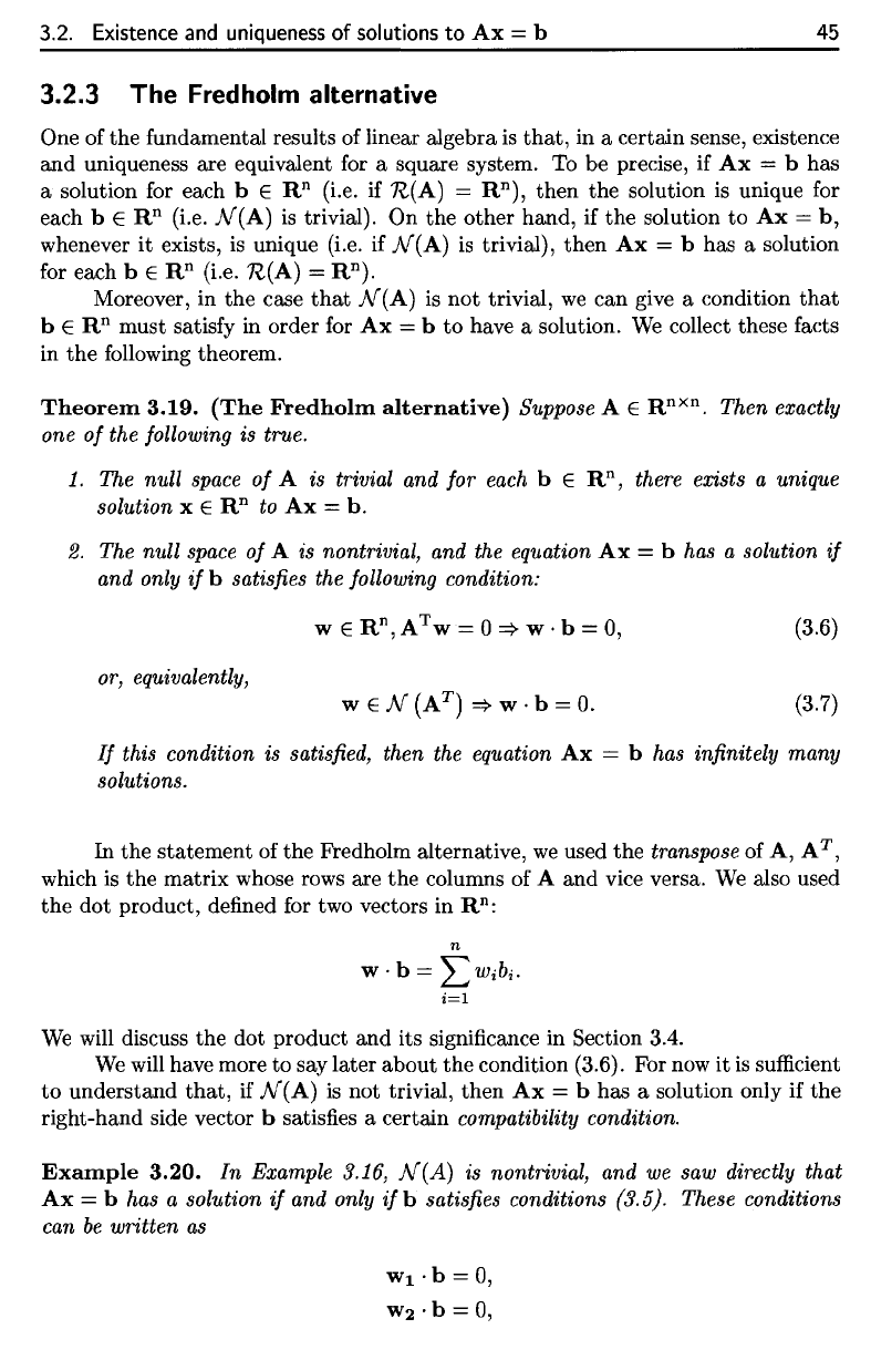
is a solution
of
the system. We have that
is one solution
of
Ax
=
b,
and
Example
3.17.
We compute the null space
of
the operator
LN
defined
in
Example
3.14.
If
LNU = 0, then u satisfies the
BVP
d
2
u
-
dx
2
=
0,
° < x < f,
du
(0)
=
0,
dx
~~(f)
=
0.
The differential equation implies that
u(x)
= C
1
x + C
2
for some constants C
1
and C
2
•
The two boundary conditions each lead to the conclusion that C
1
=
0,-
however, the constant C
2
can have any value and both the differential equation
and the two boundary conditions will
be
satisfied. This shows that every constant
function
u(x)
= C
2
satisfies
LNu
=
0.
That is, the null space
of
LN
is the space
of
constant functions.
Since
the
null space of
LN
is not trivial,
we
know from
the
above discussion
that
the
operator equation LNU = f cannot have a unique
solution-if
there is one
solution, there must in fact be infinitely many. However, since
the
null space is
the
set of constant functions, all solutions
to
LNu
= f differ by a constant.
Example
3.18.
The null space
of
the operator LD defined in Example 3.15 is
trivial.
To
see this, the reader should note that the differential equation
d
2
u
--=0
dx
2
again implies that
u(x)
= C
1
x + C
2
,-
however, now the boundary conditions
u(O)
=
u(f)
= ° force C
1
= C
2
=
O.
Therefore, the only solution
of
LDU
= 0 is the zero
function.
Since
the
null space of LD
is
trivial,
we
see
that
LDu
= f has
at
most one
solution for any right-hand side
f.
3.2. Existence
and
uniqueness
of
solutions
to Ax = b 45
3.2.3
The
Fredholm alternative
One
of the
fundamental results
of
linear algebra
is
that,
in a
certain sense, existence
and
uniqueness
are
equivalent
for a
square
system.
To be
precise,
if Ax
—
b has
a
solution
for
each
b G
R
n
(i.e.
if
7£(A)
=
R
n
),
then
the
solution
is
unique
for
each
b 6
R
n
(i.e.
A/"(A)
is
trivial).
On the
other hand,
if the
solution
to Ax = b,
whenever
it
exists,
is
unique (i.e.
if
A/"(A)
is
trivial), then
Ax = b has a
solution
for
each
b 6
R
n
(i.e.
ft(A) =
R
n
).
Moreover,
in the
case
that
A/"(A)
is not
trivial,
we can
give
a
condition
that
b G
R
n
must satisfy
in
order
for Ax = b to
have
a
solution.
We
collect these facts
in
the
following
theorem.
Theorem
3.19. (The
Fredholm
alternative)
Suppose
A 6
R
nxn
.
Then
exactly
one of the
following
is
true.
1.
The
null
space
of A is
trivial
and for
each
b G
R
n
,
there exists
a
unique
solution
x G
R
n
to Ax
=
b.
2. The
null
space
of
A is
nontrivial,
and the
equation
Ax = b has a
solution
if
and
only
if
b
satisfies
the
following
condition:
We
will
discuss
the dot
product
and its
significance
in
Section 3.4.
We
will
have more
to say
later
about
the
condition
(3.6).
For now it is
sufficient
to
understand
that,
if
-A/"(A)
is not
trivial, then
Ax = b has a
solution only
if the
right-hand side vector
b
satisfies
a
certain
compatibility
condition.
Example
3.20.
In
Example 3.16,
J\f(A)
is
nontrivial,
and we saw
directly
that
Ax = b has a
solution
if and
only
ifb
satisfies
conditions (3.5). These conditions
can be
written
as
or,
equivalently,
If
this condition
is
satisfied,
then
the
equation
Ax = b has
infinitely
many
solutions.
In the
statement
of the
Fredholm alternative,
we
used
the
transpose
of A,
A
T
,
which
is the
matrix whose rows
are the
columns
of A and
vice versa.
We
also used
the dot
product,
defined
for two
vectors
in
R
n
:
3.2. Existence
and
uniqueness
of
solutions
to
Ax
= b 45
3.2.3 The Fredholm alternative
One of
the
fundamental results of linear algebra is
that,
in a certain sense, existence
and
uniqueness are equivalent for a square system. To be precise,
if
Ax
= b has
a solution for each
bERn
(i.e. if
R(A)
=
Rn),
then
the
solution is unique for
each
bERn
(i.e.
N(A)
is trivial).
On
the
other
hand, if
the
solution
to
Ax
=
b,
whenever
it
exists, is unique (i.e. if
N(A)
is
trivial),
then
Ax
= b has a solution
for each
bERn
(i.e.
R(A)
= Rn).
Moreover, in
the
case
that
N(A)
is
not
trivial,
we
can give a condition
that
bERn
must satisfy in order for
Ax
= b
to
have a solution.
We
collect these facts
in
the
following theorem.
Theorem
3.19.
(The
Fredholm
alternative)
Suppose A E Rnxn. Then exactly
one
of
the following is true.
1.
The null space
of
A is trivial and for each b
ERn,
there exists a unique
solution x
E R
n
to
Ax
=
b.
2.
The null space
of
A is nontrivial, and the equation
Ax
= b has a solution
if
and only
if
b satisfies the following condition:
wE
Rn,
ATw
= 0
:::}
W·
b = 0,
(3.6)
or,
equivalently,
(3.7)
If
this condition is satisfied, then the equation
Ax
= b has infinitely many
solutions.
In
the
statement
of
the
Fredholm alternative,
we
used
the
transpose of
A,
AT,
which is
the
matrix
whose rows are
the
columns of A
and
vice versa. We also used
the
dot product, defined for two vectors in Rn:
n
w·
b =
LWibi.
i=l
We
will discuss the dot product
and
its significance in Section 3.4.
We
will have more
to
say later
about
the
condition (3.6). For now
it
is sufficient
to
understand
that,
if
N(A)
is
not trivial,
then
Ax
= b has a solution only
if
the
right-hand side vector b satisfies a certain compatibility condition.
Example
3.20.
In
Example 3.16,
N(A)
is nontrivial, and we saw directly that
Ax
= b has a solution
if
and only
if
b satisfies conditions
{3.5}.
These conditions
can
be
written
as
WI'
b =
0,
W2'
b =
0,
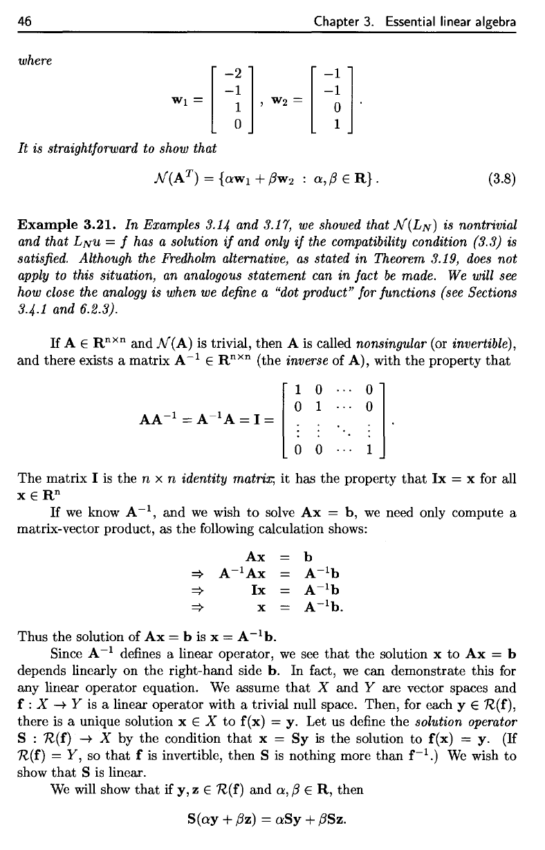
46
Chapter
3.
Essential linear algebra
where
Example
3.21.
In
Examples 3.14
and
3.17,
we
showed
that
A/"(L/v)
is
nontrivial
and
that
L^u
= f has a
solution
if and
only
if the
compatibility
condition (3.3)
is
satisfied.
Although
the
Fredholm
alternative,
as
stated
in
Theorem
3.19,
does
not
apply
to
this situation,
an
analogous
statement
can in
fact
be
made.
We
will
see
how
close
the
analogy
is
when
we
define
a
"dot product"
for
functions (see Sections
3.4.1
and
6.2.3).
If
A
e
R
nxn
and
JV(A)
is
trivial, then
A is
called nonsingular
(or
invertible),
and
there exists
a
matrix
A"
1
G
R
nxn
(the
inverse
of A),
with
the
property
that
Thus
the
solution
of Ax = b is x
=
A
x
b.
Since
A"
1
defines
a
linear operator,
we see
that
the
solution
x to Ax = b
depends linearly
on the
right-hand side
b. In
fact,
we can
demonstrate this
for
any
linear
operator
equation.
We
assume
that
X and Y are
vector
spaces
and
f : X
-»
Y is a
linear operator with
a
trivial null space. Then,
for
each
y €
7?.(f),
there
is a
unique solution
x
e
X to f
(x)
= y. Let us
define
the
solution
operator
S :
7£(f)
-»
X by the
condition
that
x = Sy is the
solution
to f
(x)
=
y. (If
K(f)
—
Y,
so
that
f is
invertible, then
S is
nothing more
than
f"
1
.)
We
wish
to
show
that
S is
linear.
We
will
show
that
if y, z
e
7£(f)
and a, ft € R,
then
It is
straightforward
to
show that
The
matrix
I is the n x n
identity
matrix;
it has the
property
that
Ix
= x for all
xeR
n
.
If
we
know
A"
1
,
and we
wish
to
solve
Ax = b, we
need only compute
a
matrix-vector
product,
as the following
calculation shows:
46
Chapter
3.
Essential linear algebra
where
It
is straightforward to show that
(3.8)
Example
3.21.
In
Examples 3.14 and 3.17, we showed that
N(LN)
is nontrivial
and that
LNu = f has a solution
if
and only
if
the compatibility condition (3.3) is
satisfied. Although the Fredholm alternative,
as
stated in Theorem 3.19,
does
not
apply to this situation, an analogous statement can in fact
be
made. We will see
how close the analogy is when
we
define a "dot product" for junctions (see Sections
3.4.1 and
6.2.3).
If
A E Rnxn and
N(A)
is trivial, then A
is
called nonsingular (or invertible),
and there exists a matrix
A-
1
E R
nxn
(the inverse of
A),
with
the
property
that
The matrix I
is
the
n x n identity matrix; it has the property
that
Ix
= x for all
x
ERn
If
we
know A
-1,
and
we
wish
to
solve
Ax
=
b,
we
need only compute a
matrix-vector product, as
the
following calculation shows:
Ax
::::}
A-lAx
::::}
Ix
::::}
x
Thus
the
solution of
Ax
= b
is
x = A -1
b.
Since A -1 defines a linear operator,
we
see
that
the solution x
to
Ax
= b
depends linearly on the right-hand side
b.
In fact,
we
can demonstrate this for
any linear operator equation.
We
assume
that
X and Y are vector spaces and
f:
X
-t
Y
is
a linear operator with a trivial null space. Then, for each y E
R(f),
there
is
a unique solution x E X
to
f(x) =
y.
Let us define the solution operator
S :
R(f)
-t
X by
the
condition
that
x =
Sy
is
the
solution to f(x) =
y.
(If
R(f)
= Y, so
that
f
is
invertible, then S
is
nothing more
than
f-1.)
We
wish
to
show
that
S
is
linear.
We
will show
that
if
y,
Z E
R(f)
and a,
(3
E
R,
then
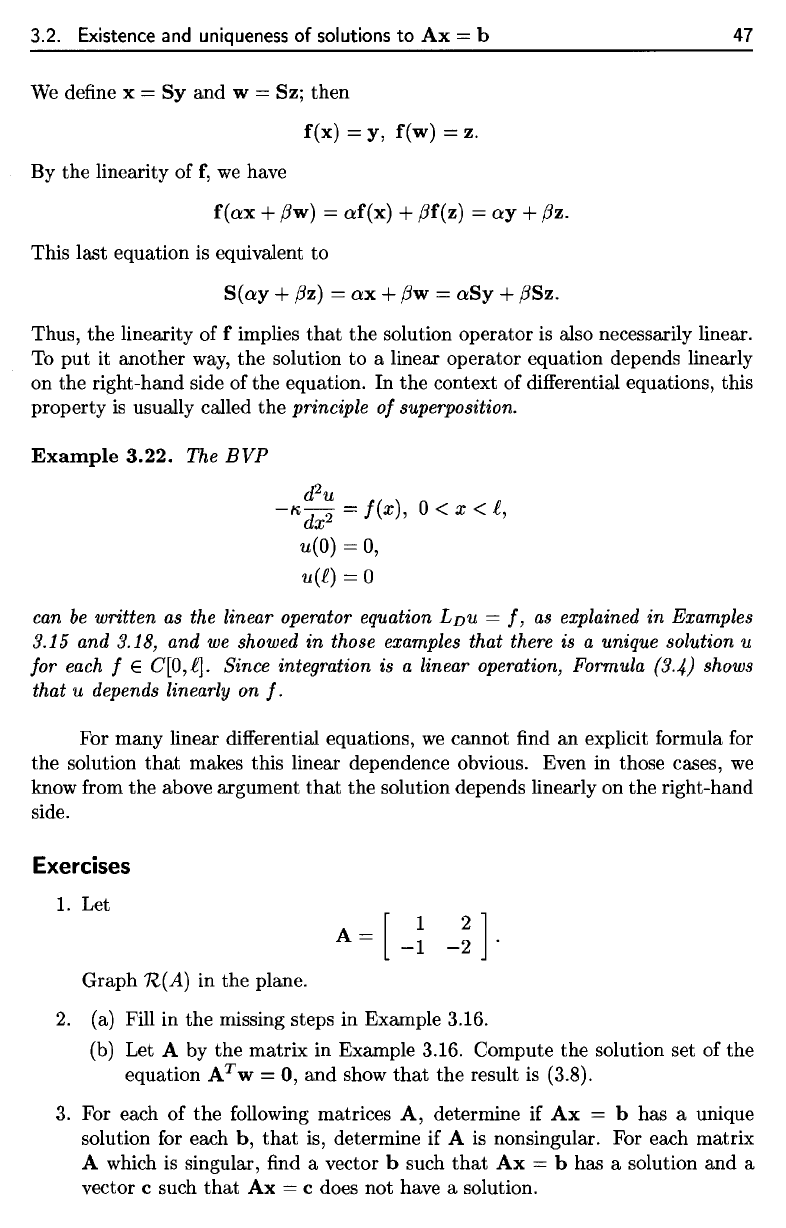
S(ay
+
(3z)
=
aSy
+ (3Sz.
3.2.
Existence
and
uniqueness
of
solutions
to Ax = b 47
We
define
x
=
Sy and w = Sz;
then
By the
linearity
of f, we
have
This
last
equation
is
equivalent
to
Thus,
the
linearity
of f
implies
that
the
solution operator
is
also necessarily linear.
To
put it
another way,
the
solution
to a
linear operator equation depends linearly
on
the
right-hand side
of the
equation.
In the
context
of
differential
equations, this
property
is
usually called
the
principle
of
superposition.
Example 3.22.
The
BVP
can
be
written
as the
linear
operator
equation
Lpu
=
/,
as
explained
in
Examples
3.15
and
3.18,
and we
showed
in
those
examples
that there
is a
unique solution
u
for
each
f
e
C[0,£].
Since integration
is a
linear operation, Formula (3.4)
shows
that
u
depends
linearly
on
f.
For
many linear
differential
equations,
we
cannot
find an
explicit formula
for
the
solution
that
makes this linear dependence obvious. Even
in
those cases,
we
know
from
the
above argument
that
the
solution depends linearly
on the
right-hand
side.
Exercises
1. Let
Graph
H(A)
in the
plane.
2.
(a)
Fill
in the
missing steps
in
Example 3.16.
(b)
Let A by the
matrix
in
Example 3.16. Compute
the
solution
set of the
equation
A
T
w
= 0, and
show
that
the
result
is
(3.8).
3. For
each
of the
following
matrices
A,
determine
if Ax
=
b has a
unique
solution
for
each
b,
that
is,
determine
if A is
nonsingular.
For
each matrix
A
which
is
singular,
find a
vector
b
such
that
Ax
=
b has a
solution
and a
vector
c
such
that
Ax = c
does
not
have
a
solution.
3.2. Existence and uniqueness
of
solutions
to
Ax
= b
47
We define x =
Sy
and
w =
Sz;
then
f(x)
=
y,
f(w)
= z.
By
the
linearity of
f,
we
have
f(ax
+ (3w) =
af(x)
+ (3f(z) =
ay
+
(3z.
This last equation is equivalent
to
S(ay
+
(3z)
=
ax
+ (3w =
aSy
+ (3Sz.
Thus,
the
linearity of f implies
that
the
solution operator is also necessarily linear.
To
put
it another way,
the
solution
to
a linear operator equation depends linearly
on the right-hand side of the equation. In
the
context of differential equations, this
property is usually called
the
principle
of
superposition.
Example
3.22.
The
BVP
d
2
u
-/1,
dx
2
= f(x), 0 < x <
f,
u(O)
= 0,
u(f) = 0
can
be
written
as
the linear operator equation
LDu
=
f,
as
explained
in
Examples
3.15 and 3.18, and
we
showed
in
those examples that there is a unique solution u
for each f E
C[O,
fl.
Since integration is a linear operation, Formula (3.4) shows
that u depends linearly on
f.
For many linear differential equations,
we
cannot find
an
explicit formula for
the
solution
that
makes this linear dependence obvious. Even in those cases,
we
know from
the
above argument
that
the
solution depends linearly on
the
right-hand
side.
Exercises
1.
Let
A=[
Graph
R(A)
in the plane.
2.
(a) Fill in
the
missing steps in Example 3.16.
(b) Let A by
the
matrix in Example 3.16. Compute
the
solution set of
the
equation
AT
w = 0,
and
show
that
the result
is
(3.8).
3. For each of
the
following matrices
A,
determine if
Ax
= b has a unique
solution for each
b,
that
is, determine if A is nonsingular. For each matrix
A which is singular, find a vector b such
that
Ax
= b has a solution
and
a
vector c such
that
Ax
= c does not have a solution.
