Gockenbach M.S. Partial Differential Equations. Analytical and Numerical Methods
Подождите немного. Документ загружается.


This page intentionally left blank
This page intentionally left blank
In
this chapter,
we
present several
different
and
interesting physical processes
that
can be
modeled
by
ODEs
or
PDEs.
For now we
restrict ourselves
to
phenomena
that
can be
described
(at
least approximately)
as
occurring
in a
single
spatial
dimension:
heat
flow or
mechanical vibration
in a
long, thin bar, vibration
of a
string,
diffusion
of
chemicals
in a
pipe,
and so
forth.
In
Chapters 5-7,
we
will
learn methods
for
solving
the
resulting
differential
equations.
In
Chapter
8, we
consider similar experiments occurring
in
multiple
spatial
dimensions.
2.1
Heat
flow
in a
bar; Fourier's
law
We
begin
by
considering
the
distribution
of
heat energy (or,
equivalently,
of
temper-
ature)
in a
long, thin bar.
We
assume
that
the
cross-sections
of the bar are
uniform,
and
that
the
temperature varies only
in the
longitudinal direction.
In
particular,
we
assume
that
the bar is
perfectly insulated, except possibly
at the
ends,
so
that
no
heat
escapes through
the
side.
By
making several
simplifying
assumptions,
we
derive
a
linear
PDE
whose solution
is the
temperature
in the bar as a
function
of
spatial
position
and
time.
We
show, when
we
treat
multiple space dimensions
in
Chapter
8,
that
if the
initial temperature
is
constant
in
each cross-section,
and if any
heat
source depends
only
on the
longitudinal coordinate, then
all
subsequent temperature distributions
depend only
on the
longitudinal coordinate. Therefore,
in
this regard, there
is
no
modeling error
in
adopting
a
one-dimensional model. (There
is
modeling error
associated with some
of the
other assumptions
we
make.)
We
will
now
derive
the
model, which
is
usually called
the
heat
equation.
We
begin
by
defining
a
coordinate system (see Figure
2.1).
The
variable
x
denotes
position
in the bar in the
longitudinal direction,
and we
assume
that
one end of the
bar is at x = 0. The
length
of the bar
will
be
£,
so the
other
end is at x = t. We
denote
by A the
area
of a
cross-section
of the
bar.
The
temperature
of the bar is
determined
by the
amount
of
heat energy
in
Chapter
2
in one
dimension
9
Modelas
s
in
one dimension
In
this chapter,
we
present several different
and
interesting physical processes
that
can be modeled by ODEs or PDEs. For now
we
restrict ourselves
to
phenomena
that
can be described
(at
least approximately) as occurring in a single spatial dimension:
heat
flow
or
mechanical vibration in a long,
thin
bar, vibration of a string, diffusion
of chemicals in a pipe,
and
so forth. In Chapters 5-7,
we
will learn methods for
solving
the
resulting differential equations.
In
Chapter
8,
we
consider similar experiments occurring in multiple spatial
dimensions.
2.1
Heat
flow
in
a
bar;
Fourier's law
We
begin by considering
the
distribution of heat energy (or, equivalently, of temper-
ature) in a long,
thin
bar.
We
assume
that
the
cross-sections of the
bar
are uniform,
and
that
the
temperature
varies only in the longitudinal direction.
In
particular,
we
assume
that
the
bar
is perfectly insulated, except possibly
at
the
ends, so
that
no heat escapes through
the
side. By making several simplifying assumptions,
we
derive a linear
PDE
whose solution
is
the
temperature in
the
bar
as a function of
spatial position
and
time.
We
show, when
we
treat
multiple space dimensions in
Chapter
8,
that
if
the
initial
temperature
is constant in each cross-section, and if any heat source depends
only on
the
longitudinal coordinate,
then
all subsequent temperature distributions
depend only on
the
longitudinal coordinate. Therefore, in this regard, there is
no modeling error in adopting a one-dimensional model. (There is modeling error
associated with some of
the
other assumptions
we
make.)
We
will now derive
the
model, which is usually called
the
heat equation.
We
begin by defining a coordinate system (see Figure 2.1).
The
variable x denotes
position in
the
bar
in
the
longitudinal direction,
and
we
assume
that
one end of
the
bar
is
at
x =
O.
The
length of
the
bar
will be
f,
so
the
other
end
is
at
x =
£.
We
denote by A
the
area
of a cross-section of the bar.
The
temperature
of
the
bar
is
determined by
the
amount of heat energy in
9
2.1. Heat flow
in a
bar; Fourier's
law 11
The
fact
that
we do not
know
EQ
causes
no
difficulty,
because
we are
going
to
model
the
change
in the
energy (and hence
temperature).
Specifically,
we
examine
the
rate
of
change, with respect
to
time,
of the
heat
energy
in the
part
of the bar
between
x and x +
Ax.
The
total
heat
in
[x,
x + Ax]
is
given
by
(2.2),
so its
rate
of
change
is
(the constant
EQ
differentiates
to
zero).
To
work with this expression,
we
need
the
following
result, which allows
us to
move
the
derivative
past
the
integral sign:
Theorem
2.1.
Let F
:
(a,b)
x [c,
d\
—>•
R and
dF/dx
be
continuous,
and
define
(f>:
(a, 6)
->•
R by
If
we
assume
that
there
are no
internal sources
or
sinks
of
heat,
the
heat
contained
in [x, x + Ax] can
change only because
heat
flows
through
the
cross-
sections
at x and x + Ax. The
rate
at
which heat
flows
through
the
cross-section
at x is
called
the
heat
flux, and is
denoted
q(x,t).
It has
units
of
energy
per
unit
area
per
unit time,
and is a
signed quantity:
if
heat energy
is flowing in the
positive
x-direction, then
q is
positive.
The net
heat entering
[x, x + Ax] at
time
t,
through
the two
cross-sections,
is
Then
0
is
continuously
differentiate,
and
That
is,
By
Theorem 2.1,
we
have
the
last
equation
follows
from
the
fundamental theorem
of
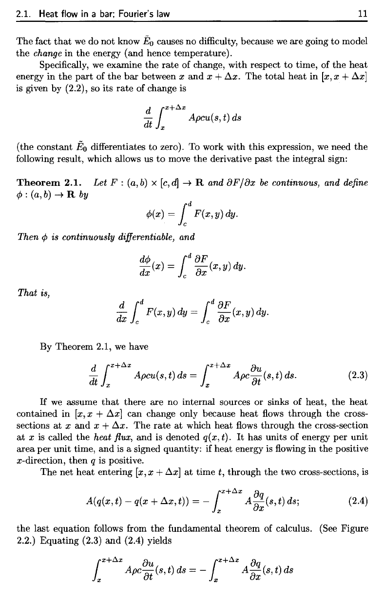
calculus. (See Figure
2.2.)
Equating (2.3)
and
(2.4) yields
2.1. Heat
flow
in
a
bar;
Fourier's
law
11
The
fact
that
we
do
not
know
Eo
causes
no
difficulty, because
we
are
going
to
model
the
change in
the
energy
(and
hence
temperature).
Specifically, we examine
the
rate
of change,
with
respect
to
time, of
the
heat
energy in
the
part
of
the
bar
between x
and
x +
~x.
The
total
heat
in
[x,
x +
~xl
is given
by
(2.2), so its
rate
of change is
d
r+tl.x
dt
ix
Apeu(s,t)ds
(the
constant
Eo
differentiates
to
zero). To work
with
this
expression,
we
need
the
following result, which allows us
to
move
the
derivative
past
the
integral sign:
Theorem
2.1.
Let F : (a,
b)
x
[e,
d]
-+
Rand
aF/ax
be
continuous, and define
¢ :
(a,
b)
-+
R by
¢(x)
=
ld
F(x,
y) dy.
Then ¢ is continuously differentiable, and
d¢
ld
aF
dx
(x) = c
ax
(x, y) dy.
That is,
d
ld
ld
aF
dx
c
F(x,y)dy=
c
ax
(x,y)dy.
By
Theorem
2.1, we have
d
r+tl.x
r+tl.x
au
dt
ix
Apcu(s, t) ds =
ix
Ape
at
(s, t) ds.
(2.3)
If
we assume
that
there
are
no internal sources
or
sinks
of
heat,
the
heat
contained in
[x,
x +
~xl
can
change only because
heat
flows
through
the
cross-
sections
at
x
and
x +
~x.
The
rate
at
which
heat
flows
through
the
cross-section
at
x
is
called
the
heat flux,
and
is denoted q(x, t).
It
has
units
of
energy
per
unit
area
per
unit
time,
and
is a signed quantity: if
heat
energy is flowing in
the
positive
x-direction,
then
q is positive.
The
net
heat
entering
[x,
x +
~xl
at
time
t,
through
the
two cross-sections,
is
r+tl.x
aq
A(q(x,
t) - q(x +
~x,
t)) = -
ix
A
ax
(s, t) ds;
(2.4)
the
last
equation
follows from
the
fundamental
theorem
of calculus. (See Figure
2.2.)
Equating
(2.3)
and
(2.4) yields
r+tl.x
au
r+tl.x
aq
ix
Ape
at
(s,t)ds
= -
ix
Aax(s,t)ds
12
Chapter
2.
Models
in one
dimension
Figure
2.2.
The
heat
flux
into
and out of a
part
of the
bar.
Naturally,
heat
will
flow
from
regions
of
higher
temperature
to
regions
of
lower
temperature; note
that
the
sign
of
du/dx
indicates whether temperature
is
increasing
or
decreasing
as x
increases,
and
hence indicates
the
direction
of
heat
flow.
We
now
make
a
simplifying
assumption, which
is
called Fourier's
law
of
heat
conduction:
the
heat
flux q is
proportional
to the
temperature
gradient,
du/dx.
We
call
the
magnitude
of the
constant
of
proportionality
the
thermal conductivity
K,
and
obtain
the
equation
or
Since
this holds
for all x and
Ax,
it
follows
that
the
integrand must
be
zero:
(The
key
point here
is
that
the
integral above equals zero over
every
small interval.
This
is
only possible
if the
integrand
is
itself zero.
If the
integrand
were
positive,
say,
at
some point
in
[0,^],
and
were continuous, then
the
integral over
a
small
interval
around
that
point
would
be
positive.)
(the
units
of K can be
determined
from
the
units
of the
heat
flux and
those
of the
temperature gradient;
see
Exercise
2.1.1).
The
negative sign
is
necessary
so
that
heat
flows
from
hot
regions
to
cold. Substituting Fourier's
law
into
the
differential
equation (2.5),
we can
eliminate
q and find a PDE for
u:
(We
have canceled
a
common
factor
of A)
Here
we
have assumed
that
K
is
constant,
which
would
be
true
if the bar
were homogeneous.
It is
possible
that
K
depends
on
x (in
which case
p and c
probably
do as
well);
then
we
obtain
We
call (2.7)
the
heat
equation.
If
the bar
contains internal sources
(or
sinks)
of
heat (such
as
chemical reac-
tions
that
produce heat),
we
collect
all
such sources into
a
single
source
function
12
Chapter
2.
Models
in
one dimension
or
l
X
+
dX
{au
a
q
}
x Ape
at
(8,
t) + A
ax
(8,
t)
d8
=
O.
Since this holds for all x and
~x,
it
follows
that
the integrand must be zero:
au
aq
Ape
at
(x, t) + A
ax
(x, t) =
0,
0 < x <
c.
(2.5)
(The key point here
is
that
the
integral above equals zero over every small interval.
This
is
only possible
if
the integrand
is
itself zero.
If
the integrand were positive,
say,
at
some point in
[0,
C),
and
were continuous, then the integral over a small
interval around
that
point would be positive.)
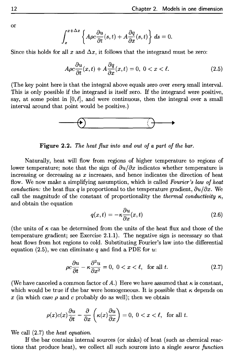
Figure
2.2. The heat flux into and out
of
a part
of
the
bar.
Naturally,
heat
will
flow
from regions of higher temperature
to
regions of
lower temperature; note
that
the sign of
au/ax
indicates whether temperature
is
increasing or decreasing as x increases, and hence indicates the direction of heat
flow.
We
now make a simplifying assumption, which
is
called Fourier's
law
of
heat
conduction:
the
heat flux q
is
proportional to
the
temperature gradient,
au/ax.
We
call the magnitude of
the
constant of proportionality
the
thermal conductivity r.,
and obtain the equation
au
q(x, t) =
-r.
ax
(x, t)
(2.6)
(the units of
r.
can be determined from
the
units of the heat flux and those of the
temperature gradient; see Exercise 2.1.1).
The
negative sign
is
necessary so
that
heat
flows
from hot regions
to
cold. Substituting Fourier's law into the differential
equation (2.5),
we
can eliminate q and find a
PDE
for u:
au
a
2
u
pc
at
-
r.
ax
2
=
0,
0 < x <
C,
for all t.
(2.7)
(We
have canceled a common factor of A.) Here
we
have assumed
that
r.
is
constant,
which would
be
true
if
the
bar
were homogeneous.
It
is
possible
that
r. depends on
x (in which case p and e probably do as well); then
we
obtain
p(x)c(x)
~~
-
:x
(r.(x)
~~)
=
0,
0 < x <
C,
for all t.
We
call (2.7) the heat equation.
If
the
bar
contains internal sources (or sinks) of heat (such as chemical reac-
tions
that
produce heat),
we
collect all such sources into a single source function
2.1. Heat flow
in a
bar; Fourier's
law 13
/(x,t)
(in
units
of
heat energy
per
unit time
per
unit
volume).
Then
the
total
heat
added
to
[x,
x + Ax]
during
the
time interval
[t,
t +
At]
is
Either
of
these boundary conditions
can be
inhomogeneous
(that
is,
have
a
nonzero
right-hand side),
and we
could,
of
course, have mixed conditions (one
end
insulated,
the
other held
at fixed
temperature).
A
boundary condition
that
specifies
the
value
of the
solution
is
called
a
Dirich-
let
condition,
while
a
condition
that
specifies
the
value
of the
derivative
is
called
a
Neumann condition.
A
problem with
a
Dirichlet condition
at one end and a
Neu-
mann condition
at the
other
is
said
to
have
mixed
boundary
conditions.
As
noted
3
The
term
homogeneous
is
used
in two
completely
different
ways
in
this section
and
throughout
the
book.
A
material
can be
(physically) homogeneous,
which
implies
that
the
coefficients
in the
differential
equations
will
be
constants.
On the
other hand,
a
linear
differential
equation
can be
(mathematically)
homogeneous,
which
means that
the right-hand
side
is
zero.
These
two
uses
of
the
word
homogeneous
are
unrelated
and
potentially
confusing,
but the
usage
is
standard
and so
the
reader must understand
from
context
the
sense
in
which
the
word
is
used.
4
Since
changing
u by an
additive constant does
not
affect
the
differential
equation,
we can as
well
use
Celsius
as the
temperature
scale
rather than
Kelvin.
(See Exercise
6.)
The
time
rate
of
change
of
this contribution
to the
total
heat energy
(at
time
t) is
The
rate
of
change
of
total
heat
in
[#,
x + Ax] is now
given
by the sum of
(2.4)
and
(2.8),
so we
obtain,
by the
above reasoning,
the
inhomogeneous
3
heat
equation
2.1.1
Boundary
and
initial
conditions
for the
heat equation
The
heat
equation
by
itself
is not a
complete model
of
heat
flow. We
must know
how
heat
flows
through
the
ends
of the
bar,
and we
must know
the
temperature
distribution
in the bar at
some initial time.
Two
possible boundary conditions
for
heat
flow in a bar
correspond
to
perfect
insulation
and
perfect thermal contact.
If the
ends
of the bar are
perfectly insulated,
so
that
the
heat
flux
across
the
ends
is
zero, then
we
have
(no
heat
flows
into
the
left
end or out of the
right end).
On the
other hand,
if
the
ends
of the bar are
kept
fixed at
temperature
zero
4
(through perfect
thermal
contact with
an ice
bath,
for
instance),
we
obtain
u(0,t)
=u(l,t]
= 0 for
alH.
2.1. Heat flow
in
a
bar;
Fourier's law
13
f(x,
t) (in units of heat energy per unit time per unit volume). Then
the
total
heat
added
to
[x,
x +
~xl
during
the
time interval
[t,
t +
~tl
is
t+.t:.t l
x
+.t:.x
it
x
Af(s,
r)
ds dr.
The
time
rate
of change of this contribution
to
the
total
heat energy
(at
time t) is
l
x
+.t:.x
x
Af(s,
t) ds.
(2.8)
The
rate
of change of
total
heat in
[x,
x +
~xl
is now given by
the
sum of (2.4) and
(2.8), so
we
obtain, by
the
above reasoning,
the
inhomogeneous
3
heat equation
au
a
2
u
pc
at
-
"'ax
2
=
f(x,t),
0<
x <
£,
for all t.
(2.9)
2.1.1 Boundary and initial conditions
for
the
heat equation
The
heat equation by itself
is
not a complete model of heat
flow.
We
must know
how heat
flows
through
the
ends of
the
bar,
and
we
must know
the
temperature
distribution in
the
bar
at
some initial time.
Two possible boundary conditions for heat
flow
in a
bar
correspond
to
perfect
insulation
and
perfect thermal contact.
If
the
ends of
the
bar
are perfectly insulated,
so
that
the
heat flux across the ends is zero,
then
we
have
au au
-K,
ax
(0, t) = 0,
-K,
ax
(£,
t)
= ° for all t
(no
heat
flows
into
the
left end or
out
of
the
right end).
On
the
other hand, if
the
ends of
the
bar
are kept fixed
at
temperature zero
4
(through perfect thermal
contact with
an
ice
bath,
for instance),
we
obtain
u(O,
t) = u(£, t) = 0 for all t.
Either of these boundary conditions can be inhomogeneous
(that
is, have a nonzero
right-hand side),
and
we
could, of course, have mixed conditions (one end insulated,
the
other held
at
fixed temperature).
A boundary condition
that
specifies
the
value of the solution
is
called a Dirich-
let condition,
while a condition
that
specifies the value
of
the
derivative is called a
Neumann condition. A problem with a Dirichlet condition
at
one end
and
a Neu-
mann
condition
at
the
other
is
said
to
have mixed boundary conditions.
As
noted
3The
term
homogeneous is used in two completely different ways in
this
section
and
throughout
the
book. A
material
can
be
(physically) homogeneous, which implies
that
the
coefficients in
the
differential equations will be constants.
On
the
other
hand, a linear differential equation
can
be
(mathematically) homogeneous, which means
that
the
right-hand side is zero. These two uses of
the
word homogeneous are
unrelated
and
potentially confusing,
but
the
usage is
standard
and
so
the
reader
must
understand
from context
the
sense in which
the
word is used.
4Since changing
u by
an
additive
constant
does
not
affect
the
differential equation,
we
can
as
well use Celsius as
the
temperature
scale
rather
than
Kelvin. (See Exercise 6.)
2.1.2 Steady-state heat flow
An
important special case modeled
by the
heat
equation
is
steady-state
heat
flow—a
situation
in
which
the
temperature
is
constant with respect
to
time (although
not
necessarily
with respect
to
space).
In
this case,
the
temperature
function
u can be
thought
of as a
function
of x
alone,
u —
u(x),
the
partial derivative with respect
to
t is
zero,
and the
differential
equation becomes
above,
we
will
also
use the
terms homogeneous
and
inhomogeneous
to
refer
to the
boundary conditions.
The
condition
u(i]
= 10 is
called
an
inhomogeneous Dirichlet
condition,
for
example.
To
completely determine
the
temperature
as a
function
of
time
and
space,
we
must know
the
temperature distribution
at
some initial time
to.
This
is an
initial
rnnAH-.i.nn.'
Putting together
the
PDE,
the
boundary conditions,
and the
initial condition,
we
obtain
an
initial-boundary value problem
(IBVP)
for the
heat
equation.
For
example, with both ends
of the bar
held
at fixed
temperatures,
we
have
the
IBVP
14
Chapter
2.
Models
in one
dimension
In
the
steady-state
case,
any
source term
/
must
be
independent
of
time (otherwise,
the
equation could
not
possibly
be
satisfied
by a
function
u
that
is
independent
of
time).
Boundary conditions have
the
same meaning
as in the
time-dependent case,
although
in the
case
of
inhomogeneous boundary conditions,
the
boundary
data
must
be
constant.
On the
other hand,
it
obviously does
not
make sense
to
impose
an
initial condition
on a
steady-state
temperature distribution.
Collecting
these observations,
we see
that
a
steady-state heat
flow
problem
takes
the
form
of a
boundary
value
problem
(BVP).
For
example,
if the
temperature
is
fixed at the two
endpoints
of the
bar,
we
have
the
following Dirichlet problem:
We
remark
that,
when only
one
spatial dimension
is
taken into account,
a
steady-
state
(or
equilibrium]
problem results
in an ODE
rather
than
a
PDE. Moreover,
these problems,
at
least
in
their simplest
form,
can be
solved directly
by two
inte-
grations. Nevertheless,
we
will
(in
Chapter
5)
devote
a
significant
amount
of
effort
14
Chapter
2.
Models
in
one
dimension
above,
we
will also use the terms homogeneous and inhomogeneous
to
refer
to
the
boundary conditions. The condition
u(£) =
10
is
called
an
inhomogeneous Dirichlet
condition, for example.
To completely determine the temperature as a function of time and space,
we
must know
the
temperature distribution
at
some initial time
to.
This
is
an
initial
condition:
u(x,
to)
=
1jJ(x),
0 < x <
£.
Putting
together the PDE, the boundary conditions, and
the
initial condition,
we
obtain an initial-boundary value problem (IBVP) for
the
heat equation. For
example, with both ends of the
bar
held
at
fixed temperatures,
we
have
the
IBVP
au a
2
u
pc
at
-
'"
ax
2
=
f(x,
t), 0 < x <
£,
t > to,
u(x,
to)
=
1jJ(x),
0 < x <
£,
u(O,
t) = 0, t >
to,
u(£, t) = 0, t >
to.
2.1.2 Steady-state heat flow
(2.10)
An important special case modeled by the heat equation
is
steady-state heat flow--a
situation in which the temperature
is
constant with respect
to
time (although not
necessarily with respect
to
space). In this case, the temperature function u can be
thought of
as
a function of x alone, u =
u(x),
the partial derivative with respect
to
t
is
zero, and the differential equation becomes
J2u
-'"
dx
2
=
f(x),
0 < x <
£.
In the steady-state case, any source term f must be independent of time (otherwise,
the
equation could not possibly be satisfied by a function u
that
is
independent of
time). Boundary conditions have
the
same meaning as in the time-dependent case,
although in
the
case of inhomogeneous boundary conditions, the boundary
data
must be constant. On
the
other hand, it obviously does not make sense
to
impose
an initial condition on a steady-state temperature distribution.
Collecting these observations,
we
see
that
a steady-state heat
flow
problem
takes
the
form of a boundary value problem (BVP). For example,
if
the temperature
is
fixed
at
the
two endpoints of
the
bar,
we
have
the
following Dirichlet problem:
J2u
-'"
dx
2
=
f(x),
0 < x <
£,
u(O)
= 0,
(2.11)
u(£)
=
O.
We
remark
that,
when only one spatial dimension
is
taken into account, a steady-
state
(or equilibrium) problem results in
an
ODE rather
than
a PDE. Moreover,
these problems,
at
least in their simplest form, can be solved directly by two inte-
grations. Nevertheless,
we
will (in Chapter
5)
devote a significant amount of effort
The
reader should notice
that
the
thermal conductivity
of the bar
does
not
affect
the
solution
in the
previous example.
This
is
because
the bar is
homogeneous
(that
is, the
thermal conductivity
of the bar is
constant
throughout).
This should
be
contrasted
with
the
next example.
2.1. Heat
flow
in a
bar; Fourier's
law 15
toward developing methods
for
solving these ODEs, since
the
techniques
can be
gen-
eralized
to
multiple
spatial
dimensions,
and
also
form
the
foundation
for
techniques
for
solving time-dependent problems.
Example
2.2.
The
thermal conductivity
of an
aluminum
alloy
is 1.5
W/(cmK).
We
will
calculate
the
steady-state temperature
of an
aluminum
bar of
length
1 m
(insulated
along
the
sides) with
its
left
end fixed at 20
degrees
Celsius
and its
right
end
fixed at 30
degrees.
If
we
write
u
=
u(x]
for the
steady-state temperature, then
u
satisfies
the BVP
(We
changed
the
units
of the
length
of the bar to
centimeters,
so as to be
consistent
with
the
units
of the
thermal conductivity.)
The
differential
equation implies that
d?u/dx
2
is
zero,
so,
integrating once,
du/dx
is
constant,
say
Example
2.3.
A
metal
bar of
length
100 cm is
manufactured
so
that
its
thermal
conductivity
is
given
by the
formula
(the
units
of
K(X]
are
W/(cmK)).
We
will
find the
steady-state temperature
of the
bar
under
the
same conditions
as in the
previous example. That
is, we
will
solve
Thus
The
boundary
condition
w(0)
=
20
implies that
C?
=
20,
and the
second
boundary
condition then
yields
Integrating
a
second
time
yields
2.1. Heat
flow
in
a
bar;
Fourier's
law
15
toward developing methods for solving these ODEs, since
the
techniques
can
be
gen-
eralized
to
multiple
spatial
dimensions,
and
also form
the
foundation for techniques
for solving time-dependent problems.
Example
2.2.
The thermal conductivity
of
an aluminum alloy is 1.5
W/(cmK).
We will calculate the steady-state temperature
of
an aluminum
bar
of
length 1 m
(insulated along the sides) with its left end fixed at
20
degrees Celsius and its right
end fixed at 30 degrees.
If
we
write u =
u(x)
for the steady-state temperature, then
u satisfies the
BVP
d
2
u
-1.5
dx
2
= 0, 0 < x < 100,
u(O)
= 20,
u(100) = 30.
(We
changed the units
of
the length
of
the
bar
to centimeters,
so
as
to
be
consistent
with the units
of
the thermal conductivity.) The differential equation implies that
d
2
u/dx
2
is zero, so, integrating once,
du/dx
is constant, say
du
dx(x)=C
1
,0<x<100.
Integrating a second time yields
The boundary condition
u(O)
=
20
implies that C
2
= 20, and the second boundary
condition then yields
Thus
1
100C
1
+
20
=
30
~ C
1
= 10.
x
u(x)
=
20
+ 10.
The
reader should notice
that
the
thermal
conductivity
of
the
bar
does
not
affect
the
solution in
the
previous example. This is because
the
bar
is homogeneous
(that
is,
the
thermal
conductivity of
the
bar
is
constant
throughout).
This should
be contrasted with
the
next example.
Example
2.3.
A metal
bar
of
length 100 cm is manufactured
so
that its thermal
conductivity is given
by
the formula
II:(X)
= 1.4 + 0.0025x, 0 < x < 100
(the units
of
lI:(x)
are
W/(cmK)).
We will find the steady-state temperature
of
the
bar
under the same conditions
as
in
the previous example. That is,
we
will solve
16
Chapter
2.
Models
in one
dimension
the
BVP
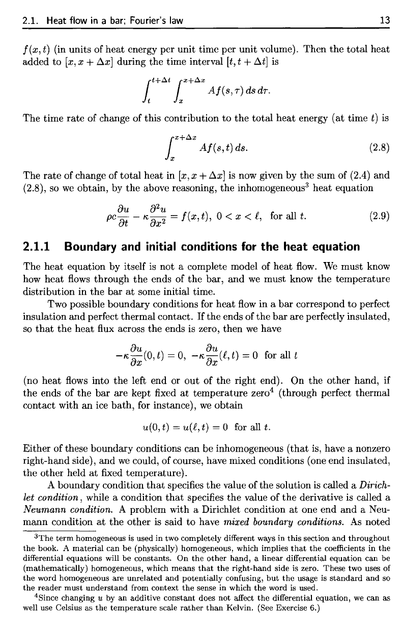
The
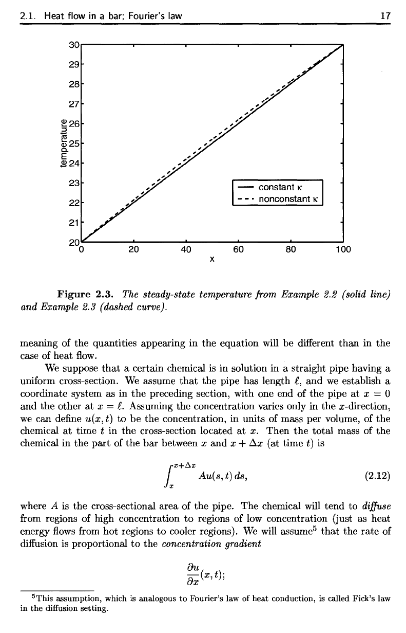
steady-state
temperatures
from
the two
previous examples
are
shown
in
Figure 2.3, which shows
that
the
heterogeneity
of the
second
bar
makes
a
small
but
discernible
difference
in the
temperature distribution.
In
both cases,
heat
energy
is
flowing
from
the
right
end of the bar to the
left,
and the
heterogeneous
bar has a
higher
thermal conductivity
at the
right end. This leads
to a
higher temperature
in
the
middle
of the
bar.
2.1.3
Diffusion
One
of the
facts
that
makes mathematics
so
useful
is
that
different
physical phe-
nomena
can
lead
to
essentially
the
same mathematical model.
In
this section
we
introduce
another experiment
that
is
modeled
by the
heat
equation.
Of
course,
the
Integrating
both
sides
of the
differential
equation
once
yields
where
C is a
constant. Equivalently,
we
have
Integrating
a
second
time
yields
Applying
the
boundary
condition
w(100)
= 30, we
obtain
With
this value
for
C,
we
have
16
the
BVP
Chapter
2.
Models
in
one
dimension
-
d~
((1.4 + 0.0025x)
:~)
=
0,
0 < x < 100,
u(O) = 20,
u(100) = 30.
Integrating both sides
of
the differential equation once yields
du
(1.4 + 0.0025x)
dx
(x) =
0,
0 < x < 100,
where 0 is a constant. Equivalently,
we
have
du
0
dx
(x) = 1.4 + 0.0025x' 0 < x <
100.
Integrating a second
time
yields
r 0
u(x)
=
u(O)
+
10
1.4 + 0.0025s ds
= 20 + r
4000
ds
10
560 + s
=
20
+
4000
In (
1
+
5:0).
Applying the boundary condition u(100) = 30,
we
obtain
0-
10
- 400 In
(~~)"
With this value for
0,
we
have
( )
_
101n(1+~)
u x -
20+
(33)
In
28
The
steady-state
temperatures
from
the
two previous examples
are
shown in
Figure 2.3, which shows
that
the
heterogeneity of
the
second
bar
makes a small
but
discernible difference in
the
temperature
distribution.
In
both
cases,
heat
energy
is
flowing from
the
right end of
the
bar
to
the
left,
and
the
heterogeneous
bar
has a
higher
thermal
conductivity
at
the
right end.
This
leads
to
a higher
temperature
in
the
middle
of
the
bar.
2.1.3
Diffusion
One
of
the
facts
that
makes
mathematics
so useful is
that
different physical phe-
nomena
can
lead
to
essentially
the
same
mathematical
model.
In
this
section we
introduce
another
experiment
that
is modeled
by
the
heat
equation.
Of
course,
the
2.1. Heat
flow
in a
bar; Fourier's
law
17
Figure
2.3.
The
steady-state temperature from
Example
2.2
(solid
line)
and
Example
2.3
(dashed
curve).
meaning
of the
quantities appearing
in the
equation
will
be
different
than
in the
case
of
heat
flow.
We
suppose
that
a
certain chemical
is in
solution
in a
straight pipe having
a
uniform
cross-section.
We
assume
that
the
pipe
has
length
t, and we
establish
a
coordinate system
as in the
preceding section, with
one end of the
pipe
at x = 0
and
the
other
at x =
1.
Assuming
the
concentration varies only
in the
^-direction,
we
can
define
u(x,
t) to be the
concentration,
in
units
of
mass
per
volume,
of the
chemical
at
time
t in the
cross-section located
at x.
Then
the
total
mass
of the
chemical
in the
part
of the bar
between
x and x +
Aar
(at
time
t) is
where
A is the
cross-sectional area
of the
pipe.
The
chemical
will
tend
to
diffuse
from
regions
of
high concentration
to
regions
of low
concentration (just
as
heat
energy
flows
from
hot
regions
to
cooler regions).
We
will
assume
5
that
the
rate
of
diffusion
is
proportional
to the
concentration gradient
5
This
assumption,
which
is
analogous
to
Fourier's
law of
heat conduction,
is
called
Pick's
law
in
the
diffusion
setting.
2.1.
Heat flow
in
a
bar;
Fourier's
law
30~--------------~------~--------------~
29
28
27
~26
::J
co
Q5
25
a.
E
224
23
22
21
20
- constant K
-
_.
nonconstant K
40
60
80
100
x
17
Figure
2.3.
The steady-state temperature from Example 2.2 (solid line)
and Example 2.3 (dashed curve).
meaning of the quantities appearing in
the
equation will be different
than
in the
case of heat
flow.
We
suppose
that
a certain chemical
is
in solution in a straight pipe having a
uniform cross-section.
We
assume
that
the pipe has length
I!,
and
we
establish a
coordinate system as in
the
preceding section, with one end of the pipe
at
x = 0
and the other
at
x =
I!.
Assuming the concentration varies only in the x-direction,
we
can define
u(x,
t) to
be
the concentration, in units of mass per volume, of the
chemical
at
time t in the cross-section located
at
x.
Then
the
total
mass of
the
chemical in the
part
of the
bar
between x
and
x +
~x
(at time t)
is
l
x+~x
x
Au(s,
t) ds,
(2.12)
where A
is
the cross-sectional area of the pipe.
The
chemical will tend to diffuse
from regions of high concentration
to
regions of low concentration (just as heat
energy
flows
from hot regions
to
cooler regions).
We
will assume
5
that
the
rate
of
diffusion
is
proportional
to
the concentration gradient
5This
assumption,
which is analogous
to
Fourier's
law of
heat
conduction,
is called
Fick's
law
in
the
diffusion
setting.