Gockenbach M.S. Partial Differential Equations. Analytical and Numerical Methods
Подождите немного. Документ загружается.

Thus
a
very small time step
is
required
for
stability,
and
this restriction
on
Af
is
imposed
by the
transient behavior
in the
system.
As
we
show below,
it is
possible
to
avoid
the
need
for
overly small time steps
in
a
stiff
system; however,
we
must
use
implicit methods. Euler's method
and the
RK
methods discussed
in
Section
4.4 are
explicit, meaning
that
the
value
w(
n+1
)
is
defined
by a
formula
involving only known quantities.
In
particular, only
u^
ap-
pears
in the
formula;
in
some explicit methods
(multistep
methods),
u^
n
~
l
\
u^
n
~
2
\
...
may
appear
in the
formula,
but
w(
n+1
)
itself does
not.
On
the
other hand,
an
implicit method
defines
u^
n+l
^
by a
formula
that
in-
volves
w(
n+1
)
itself
(as
well
as
u^
and
possibly earlier computed values
of u).
This
means
that,
at
each step
of the
iteration,
an
algebraic equation (possibly nonlinear)
must
be
solved
to find the
value
of
u(
n+1
).
In
spite
of
this additional computational
expense,
implicit methods
are
useful
because
of
their improved stability properties.
4.5.2
The
backward
Euler
method
The
simplest implicit method
is the
backward
Euler method. Recall
that
Euler's
method
for the
IVP
118
Chapter
4.
Essential ordinary differential equations
It
follows
that
and, similarly,
Clearly,
the
computation depends critically
on
If
one of
these quantities
is
larger
than
1,
the
corresponding component
will
grow
exponentially
as the
iteration progresses.
At the
very least,
for
stability
(that
is, to
avoid spurious
exponential
growth),
we
need
The first
inequality determines
the
restriction
on At, and a
little algebra shows
that
we
must have
118
It
follows
that
and, similarly,
Chapter
4. Essential ordinary differential
equations
u~n)
=
(1
- 10
7
b.t)
U~n-l)
=
(1
- 10
7
b.t)2
U~n-2)
=
(1-10
7
b.t)3
U~n-3)
= ... =
(1
-
10
7
b.tt
uiO)
=
(1
- 10
7
b.tt
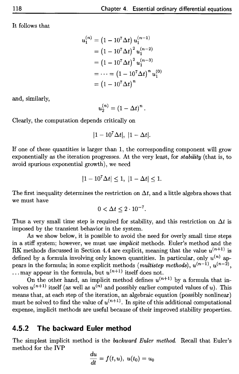
Clearly,
the
computation depends critically on
11
-
10
7
b.tl,
11
- b.tl·
If
one of these quantities is larger
than
1,
the
corresponding component will grow
exponentially as
the
iteration progresses. At
the
very least, for stability
(that
is,
to
avoid spurious exponential growth),
we
need
11
-10
7
b.tl
:::;
1,
11-
b.tl
:::;
1.
The
first inequality determines
the
restriction on b.t,
and
a little algebra shows
that
we
must have
o <
b.t
:::;
2 .
10-
7
.
Thus
a very small time step
is
required for stability,
and
this restriction on
b.t
is
imposed by
the
transient behavior in
the
system.
As
we
show below,
it
is possible
to
avoid
the
need for overly small time steps
in a stiff system; however,
we
must use implicit methods. Euler's method
and
the
RK methods discussed in Section 4.4 are explicit, meaning
that
the
value u(n+l)
is
defined by a formula involving only known quantities. In particular, only urn) ap-
pears in
the
formula; in some explicit methods (multistep methods),
u(n-I),
u(n-2),
...
may appear in
the
formula,
but
u(n+l) itself does not.
On
the
other hand,
an
implicit method defines u(n+l) by a formula
that
in-
volves
u(n+l) itself (as well as urn) and possibly earlier computed values of
u).
This
means
that,
at
each step of
the
iteration, an algebraic equation (possibly nonlinear)
must
be
solved
to
find
the
value of u(n+l). In spite of this additional computational
expense, implicit methods are useful because of their improved stability properties.
4.5.2 The
backward
Euler method
The
simplest implicit method is
the
backward Euler method. Recall
that
Euler's
method for
the
IVP
du
dt
=
f(t,
u), u(to) =
Uo
This
method
is
indeed implicit.
It is
necessary
to
solve
the
equation (4.38)
for
u
n+
i.
In the
case
of a
nonlinear
ODE (or a
system
of
nonlinear ODEs), this
may be
difficult
(requiring
a
numerical root-finding algorithm such
as
Newton's method).
However,
it is not
difficult
to
implement
the
backward
Euler
method
for a
linear
system.
We
illustrate this
for the
linear, constant-coefficient system:
4.5.
Stiff
systems
of
ODEs
119
was
derived
from
the
equivalent formulation
by
applying
the
left-endpoint
rule
for
quadrature:
The
result
is
(see
Section 4.4.1).
To
obtain
the
backward Euler method,
we
apply
the
right-hand
rule,
instead.
The
result
is
The
backward Euler method takes
the
form
Example
4.12.
Applying
the
backward
Euler method
to the
simple
example
(4-37)
gives
some insight into
the
difference
between
the
implicit
and
explicit
methods.
We
obtain
the
following
iteration
for the first
component:
4.5. Stiff systems of ODEs 119
was derived from the equivalent formulation
by applying
the
left-endpoint rule for quadrature:
lb
hex)
dx
==
h(a)(b -
a).
The result
is
U
n
+1
=
Un
+
Atf(tn,
Un)
(see Section 4.4.1). To obtain
the
backward Euler method,
we
apply the right-hand
rule,
lb
hex)
dx
==
h(b)(b
-
a),
instead. The result
is
(4.38)
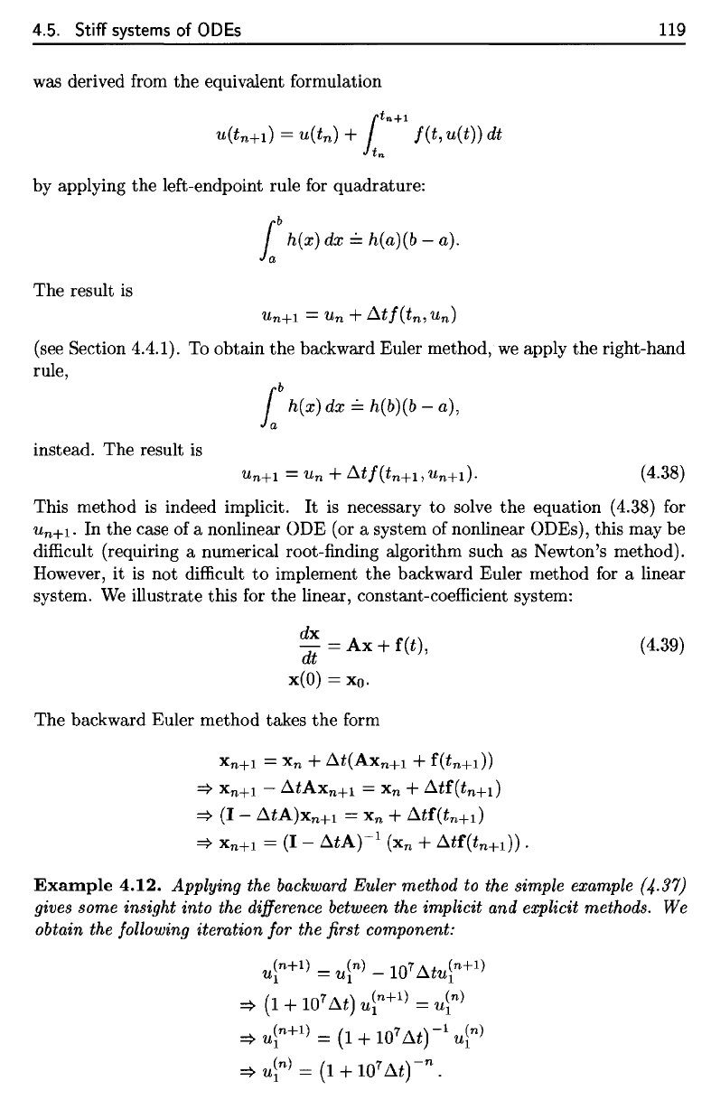
This method
is
indeed implicit.
It
is
necessary
to
solve
the
equation
(4.38)
for
U
n
+1.
In the case of a nonlinear ODE (or a system of nonlinear ODEs), this may be
difficult (requiring a numerical root-finding algorithm such as Newton's method).
However, it
is
not difficult
to
implement the backward Euler method for a linear
system.
We
illustrate this for
the
linear, constant-coefficient system:
dx
dt =
Ax
+ f(t),
x(O)
=
Xo.
The backward Euler method takes
the
form
X
n
+1
=
Xn
+ At(Axn+1 +
f(t
n
+
1
))
=}
X
n
+1
- AtAxn+1 =
Xn
+
Atf(tn+d
=}
(1
-
AtA)xn+l
=
Xn
+
Atf(t
n
+
1
)
=}
Xn+1
=
(1
-
AtA)-l
(x
n
+
Atf(tn+d)
.
(4.39)
Example
4.12.
Applying the backward Euler method to the simple example (4.37)
gives some insight into the difference between the implicit and explicit methods. We
obtain the following iteration for the first component:
(n+1)
_ (n) _
107
At
(n+1)
U
1
-
U
1
~
U
1
=}
(1
+ 10
7
At)
u~n+1)
=
ui
n
)
=}
ui
n
+1) =
(1
+ 10
7
At)
-1
ui
n
)
=}
ui
n
) =
(1
+ 10
7
At)
-n
.
120
Chapter
4.
Essential
ordinary
differential
equations
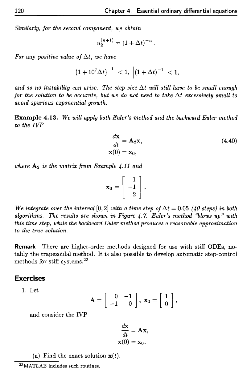
and
so no
instability
can
arise.
The
step size
A£
will still have
to be
small enough
for
the
solution
to be
accurate,
but we do not
need
to
take
Ai
excessively small
to
avoid
spurious exponential growth.
Example
4.13.
We
will
apply
both
Euler's method
and the
backward
Euler
method
to
the
IVP
and
consider
the IVP
23
MATLAB
includes such
routines.
where
A.%
is the
matrix from Example
4-11
o,nd
Similarly,
for the
second component,
we
obtain
For any
positive value
of
A£
;
we
have
We
integrate over
the
interval
[0,2]
with
a
time step
of
At
—
0.05
(40
steps)
in
both
algorithms.
The
results
are
shown
in
Figure
4-7-
Euler's method
"blows
up"
with
this time step, while
the
backward
Euler method produces
a
reasonable approximation
to
the
true solution.
Remark
There
are
higher-order methods designed
for use
with
stiff
ODEs,
no-
tably
the
trapezoidal method.
It is
also
possible
to
develop
automatic
step-control
methods
for
stiff
systems.
23
Exercises
1. Let
(a)
Find
the
exact solution
x(£).
120
Chapter
4.
Essential ordinary differential equations
Similarly, for the second component,
we
obtain
For any positive value
of
ilt,
we
have
and
so
no instability can arise. The step size
ilt
will still have to
be
small enough
for the solution to
be
accurate, but
we
do
not
need to take
ilt
excessively small to
avoid spurious exponential growth.
Example
4.13.
We will apply both Euler's method and the backward Euler method
to the
IVP
dx
dt = A
2
x,
( 4.40)
x(O)
= xo,
where
A2
is the matrix from Example 4.11 and
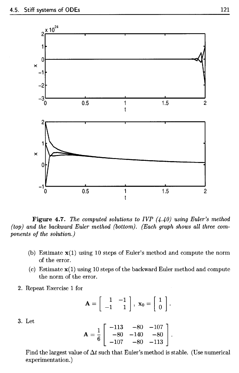
We integrate over the interval
[0,2) with a time step
of
ilt
= 0.05 (40 steps) in
both
algorithms. The results
are
shown in Figure
4.7.
Euler's method "blows up" with
this time step, while the backward Euler method produces a reasonable approximation
to the true solution.
Remark There are higher-order methods designed for use with stiff ODEs, no-
tably
the
trapezoidal method.
It
is also possible
to
develop automatic step-control
methods for stiff systems.
23
Exercises
1. Let
and
consider
the
IVP
A=[
dx
dt =
Ax,
x(O)
= xo.
(a) Find
the
exact solution
x(t).
23MATLAB includes such routines.
4.5.
Stiff
systems
of
ODEs
121
Figure
4.7.
The
computed solutions
to
IVP
(4-40)
using Euler's method
(top)
and the
backward
Euler
method
(bottom).
(Each
graph
shows
all
three
com-
ponents
of the
solution.)
(b)
Estimate
x(l) using
10
steps
of
Euler's method
and
compute
the
norm
of
the
error.
(c)
Estimate
x(l) using
10
steps
of the
backward Euler method
and
compute
the
norm
of the
error.
2.
Repeat Exercise
1 for
3. Let
Find
the
largest value
of
At
such
that
Euler's method
is
stable. (Use numerical
experimentation.)
4.5. Stiff systems of ODEs
121
0
x
-1
-2
-3
0 0.5
1.5
2
2
x
1l
0,
-1
0
0.5
1.5 2
Figure
4.7.
The computed solutions to
IVP
(4.40) using Euler's method
(top) and the backward Euler method (bottom). (Each graph shows all three com-
ponents
of
the solution.)
(b)
Estimate
x(l)
using 10 steps of Euler's
method
and
compute
the
norm
of
the
error.
(c)
Estimate
x(l)
using
10
steps of
the
backward Euler method
and
compute
the
norm
of
the
error.
2.
Repeat
Exercise 1 for
3. Let
A =
~
-80
-140
-80
.
[
-113
-80
-107]
-107
-80
-113
Find
the
largest value of
Ilt
such
that
Euler's method
is
stable. (Use numerical
experimentation. )
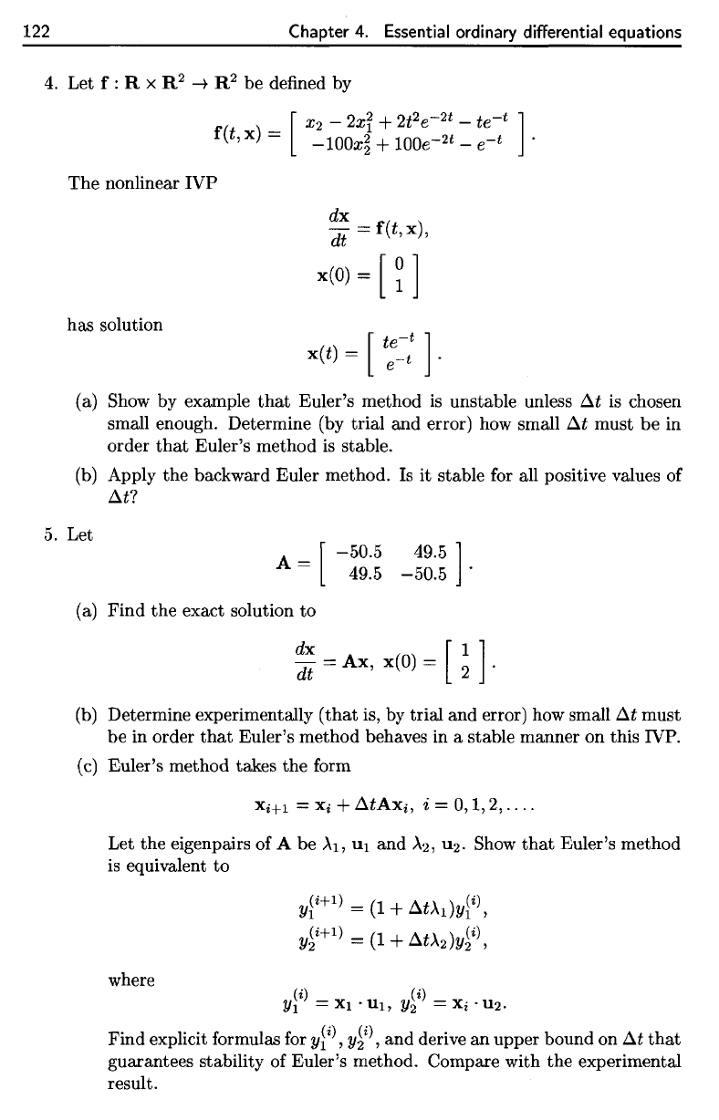
122
Chapter
4.
Essential
ordinary
differential
equations
4.
Let f : R x
R
2
->•
R
2
be
defined
by
The
nonlinear
IVP
has
solution
(a)
Show
by
example
that
Euler's
method
is
unstable unless
At is
chosen
small enough. Determine
(by
trial
and
error)
how
small
At
must
be in
order
that
Euler's method
is
stable.
(b)
Apply
the
backward
Euler
method.
Is it
stable
for all
positive values
of
At?
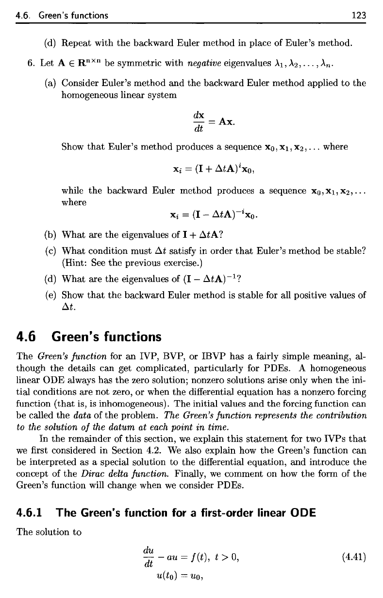
5. Let
(a)
Find
the
exact solution
to
(b)
Determine experimentally
(that
is, by
trial
and
error)
how
small
At
must
be
in
order
that
Euler's method behaves
in a
stable manner
on
this IVP.
(c)
Euler's
method
takes
the
form
Let the
eigenpairs
of A be
AI,
ui
and
A2,
112.
Show
that
Euler's method
is
equivalent
to
where
Find explicit
formulas
for
y^',
y%
, and
derive
an
upper bound
on At
that
guarantees stability
of
Euler's method. Compare with
the
experimental
rpsiilt.
122
Chapter
4.
Essential ordinary differential equations
4.
Let
f:
R x R2 -+ R2
be
defined by
The
nonlinear
IVP
dx
dt =
f(t,x),
x(o) = [
~
]
has
solution
[
te-t
]
x(t) =
e-
t
.
(a) Show by example
that
Euler's method is unstable unless
D..t
is chosen
small enough. Determine (by
trial
and
error) how small
D..t
must
be
in
order
that
Euler's
method
is
stable.
(b) Apply
the
backward Euler method. Is
it
stable for all positive values of
D..t?
5.
Let
A =
[-50.5
49.5 ]
49.5
-50.5
.
(a)
Find
the
exact solution
to
~:
=
Ax,
x(O) = [
~
] .
(b) Determine experimentally
(that
is, by trial
and
error) how small
D..t
must
be
in order
that
Euler's
method
behaves in a stable manner
on
this IVP.
(c) Euler's
method
takes
the
form
Xi+1
=
Xi
+ D..tAxi, i =
0,1,2,
....
Let
the
eigenpairs
of
A
be
.A1,
U1
and
.A2,
U2.
Show
that
Euler's
method
is equivalent
to
where
y~i+l)
=
(1
+
D..t.Ady~i),
y~i+l)
=
(1
+
D..t.A2)y~i),
(i) _ (i) _
YI
-
Xl
.
UI,
Y2
-
Xi
.
U2·
Find
explicit formulas for
y~i), y~i),
and
derive
an
upper bound
on
D..t
that
guarantees stability of Euler's method. Compare with
the
experimental
result.
4.6
Green's
functions
The
Green's
function
for an
IVP,
BVP,
or
IBVP
has a
fairly
simple meaning,
al-
though
the
details
can get
complicated, particularly
for
PDEs.
A
homogeneous
linear
ODE
always
has the
zero solution; nonzero
solutions
arise
only when
the
ini-
tial conditions
are not
zero,
or
when
the
differential
equation
has a
nonzero
forcing
function
(that
is, is
inhomogeneous).
The
initial values
and the
forcing
function
can
be
called
the
data
of the
problem.
The
Green's
function
represents
the
contribution
to the
solution
of the
datum
at
each
point
in
time.
In the
remainder
of
this
section,
we
explain
this
statement
for two
IVPs
that
we
first
considered
in
Section 4.2.
We
also explain
how the
Green's
function
can
be
interpreted
as a
special solution
to the
differential
equation,
and
introduce
the
concept
of the
Dirac
delta
function. Finally,
we
comment
on how the
form
of the
Green's
function
will
change when
we
consider PDEs.
4.6.
Green's
functions
123
(d)
Repeat with
the
backward
Euler
method
in
place
of
Euler's method.
6. Let A €
R
nxn
be
symmetric with
negative
eigenvalues
AI,
A2,...,
A
n
.
(a)
Consider Euler's method
and the
backward Euler method applied
to the
homogeneous linear system
Show
that
Euler's
method produces
a
sequence
xo,xi,X2,...
where
while
the
backward Euler method produces
a
sequence
x
0
,xi,x
2
,...
where
(b)
What
are the
eigenvalues
of I +
AtA?
(c)
What condition must
At
satisfy
in
order
that
Euler's method
be
stable?
(Hint:
See the
previous exercise.)
(d)
What
are the
eigenvalues
of (I
—
At
A)"
1
?
(e)
Show
that
the
backward Euler method
is
stable
for all
positive values
of
At.
4.6.1
The
Green's
function
for a
first-order linear
ODE
The
solution
to
4.6. Green's functions
123
(d) Repeat with
the
backward Euler method in place of Euler's method.
6.
Let A E R
nxn
be symmetric with negative eigenvalues Al,
A2,
...
,
An.
(a) Consider Euler's method
and
the
backward Euler method applied
to
the
homogeneous linear system
dx
dt =
Ax.
Show
that
Euler's method produces a sequence
XO,
Xl,
X2,
...
where
while
the
backward Euler method produces a sequence
Xo,
Xl,
X2,
...
where
Xi
= (I -
AtA)-ixo.
(b)
What
are
the
eigenvalues of 1 +
AtA?
(c)
What
condition must
At
satisfy in order
that
Euler's method be stable?
(Hint: See
the
previous exercise.)
(d)
What
are
the
eigenvalues of (I -
AtA)-l?
(e) Show
that
the
backward Euler method is stable for all positive values of
At.
4.6 Green's functions
The
Green's function for
an
IVP, BVP, or IBVP has a fairly simple meaning, al-
though
the
details can get complicated, particularly for PDEs. A homogeneous
linear
ODE always has
the
zero solution; nonzero solutions arise only when
the
ini-
tial conditions are
not
zero,
or
when
the
differential equation has a nonzero forcing
function
(that
is,
is
inhomogeneous).
The
initial values
and
the
forcing function can
be
called the data of
the
problem. The Green's function represents the contribution
to the solution
of
the datum at
each
point in time.
In
the
remainder of this section,
we
explain this
statement
for two
IVPs
that
we
first considered in Section 4.2.
We
also explain how
the
Green's function can
be
interpreted as a special solution
to
the
differential equation, and introduce
the
concept of
the
Dirac delta function. Finally,
we
comment on how
the
form of
the
Green's function will change when
we
consider PDEs.
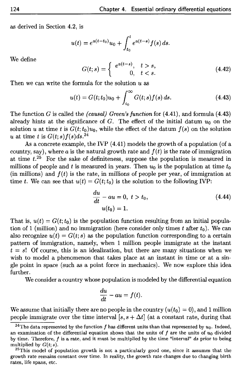
4.6.1
The
Green's function for a first-order linear
ODE
The
solution
to
du
dt - au
=
f(t),
t>
0,
(4.41)
u(to) =
uo,
124
Chapter
4.
Essential ordinary differential equations
as
derived
in
Section
4.2,
is
The
function
G is
called
the
(causal)
Green's
function
for
(4.41),
and
formula (4.43)
already hints
at the
significance
of G. The
effect
of the
initial datum
UQ
on the
solution
u at
time
t is
G(t]
to)uo,
while
the
effect
of the
datum
f(s)
on the
solution
u
at
time
t is
G(t]
s)/(s)ds.
24
As
a
concrete example,
the
IVP
(4.41) models
the
growth
of a
population
(of a
country,
say),
where
a is the
natural growth
rate
and
f(t)
is the
rate
of
immigration
at
time
t.
25
For the
sake
of
definiteness,
suppose
the
population
is
measured
in
millions
of
people
and t is
measured
in
years. Then
UQ
is the
population
at
time
to
(in
millions)
and
f(t)
is the
rate,
in
millions
of
people
per
year,
of
immigration
at
time
t. We can see
that
u(t)
=
G(t;to)
is the
solution
to the
following
IVP:
We
define
Then
we can
write
the
formula
for the
solution
u as
That
is,
u(t)
=
G(t;to)
is the
population
function
resulting
from
an
initial popula-
tion
of 1
(million)
and no
immigration (here consider only times
t
after
to).
We can
also recognize
u(t)
=
G(t;
s)
as the
population
function
corresponding
to a
certain
pattern
of
immigration, namely, when
1
million people immigrate
at the
instant
t =
si
Of
course, this
is an
idealization,
but
there
are
many situations when
we
wish
to
model
a
phenomenon
that
takes
place
at an
instant
in
time
or at a
sin-
gle
point
in
space (such
as a
point
force
in
mechanics).
We now
explore this idea
further.
We
consider
a
country whose population
is
modeled
by the
differential
equation
We
assume
that
initially there
are no
people
in the
country
(u(to)
=
0),
and 1
million
people
immigrate over
the
time interval
[s,s
+
At]
(at a
constant
rate,
during
that
24
The
data
represented
by the
function
/ has
different
units than
that
represented
by
UQ.
Indeed,
an
examination
of the
differential
equation shows
that
the
units
of / are the
units
of
UQ
divided
by
time. Therefore,
/ is a
rate,
and it
must
be
multiplied
by the
time "interval"
ds
prior
to
being
multiplied
by
G(t;
s).
25
This
model
of
population growth
is not a
particularly good one, since
it
assumes
that
the
growth
rate remains constant over time.
In
reality,
the
growth rate changes
due to
changing birth
rates,
life
spans, etc.
124
Chapter
4.
Essential ordinary differential equations
as derived in Section 4.2,
is
We define
u(t) =
ea(t-to)UO
+
rt
ea(t-s)
f(s) ds.
lto
(j(t;s) = e , s,
{
a(t-s)
t>
0,
t < s.
Then
we
can
write
the
formula for
the
solution u as
u(t) = (j(t; to)uo +
{'XI
(j(t;
s)f(s)
ds.
lto
(4.42)
(4.43)
The
function
(j
is called
the
(causal)
Green's
function for (4.41),
and
formula (4.43)
already
hints
at
the
significance of
(j.
The
effect
of
the
initial
datum
Uo
on
the
solution u
at
time
t
is
(j(t; to)uo, while
the
effect
of
the
datum
f(s)
on
the
solution
u
at
time
t is (j(t; s)f(s)ds.
24
As a concrete example,
the
IVP
(4.41) models
the
growth
of
a
population
(of a
country, say), where a is
the
natural
growth
rate
and
f(t)
is
the
rate
of
immigration
at
time
t.
25
For
the
sake
of
definiteness, suppose
the
population
is measured in
millions of people
and
t is measured
in
years.
Then
Uo
is
the
population
at
time
to
(in millions)
and
f(t) is
the
rate,
in
millions of people
per
year,
of
immigration
at
time
t. We
can
see
that
u(t) = (j(t;
to)
is
the
solution
to
the
following IVP:
du
- - au = 0 t >
to,
dt '
(4.44)
u(to) = 1.
That
is, u(t) = (j(t;
to)
is
the
population
function resulting from
an
initial popula-
tion
of
1 (million)
and
no immigration (here consider only times t after to). We
can
also recognize u(t) = (j(t;
s)
as
the
population
function corresponding
to
a
certain
pattern
of immigration, namely, when 1 million people immigrate
at
the
instant
t =
s!
Of
course,
this
is
an
idealization,
but
there
are
many
situations
when we
wish
to
model a phenomenon
that
takes place
at
an
instant
in
time
or
at
a sin-
gle
point
in space (such
as
a point force in mechanics). We now explore
this
idea
further.
We consider a
country
whose
population
is modeled by
the
differential
equation
du
dt
- au = f(t).
We assume
that
initially
there
are
no
people in
the
country
(u(to) = 0),
and
1 million
people
immigrate
over
the
time
interval
[s,
s + 6.tj
(at
a
constant
rate,
during
that
24The
data
represented by
the
function f has different
units
than
that
represented by
Uo.
Indeed,
an
examination
of
the
differential equation shows
that
the
units
of
f are
the
units
of
Uo
divided
by time. Therefore,
f is a rate,
and
it
must
be multiplied by
the
time
"interval" ds
prior
to
being
multiplied by
G(t;
s).
25This model
of
population growth is
not
a
particularly
good one, since
it
assumes
that
the
growth
rate
remains
constant
over time. In reality,
the
growth
rate
changes due
to
changing
birth
rates,
life spans, etc.
4.6. Green's
functions
125
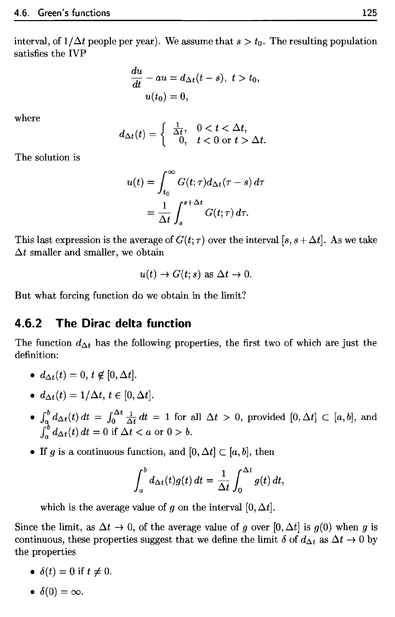
interval,
of
I/At
people
per
year).
We
assume
that
s >
to.
The
resulting population
satisfies
the
IVP
which
is the
average value
of g on the
interval
[0,
At].
Since
the
limit,
as At
->•
0, of the
average value
of g
over
[0, At] is
<?(0)
when
g is
continuous,
these properties suggest
that
we
define
the
limit
6 of
d&
t
as At
—^
0 by
the
properties
where
The
solution
is
This
last
expression
is the
average
of
G(t;
r]
over
the
interval
[s, s +
At].
As we
take
At
smaller
and
smaller,
we
obtain
But
what
forcing
function
do we
obtain
in the
limit?
4.6.2
The
Dirac delta function
The
function
d&t
has the
following
properties,
the first two of
which
are
just
the
definition:
4.6. Green's functions
125
interval, of
1/
D..t
people per year). We a.ssume
that
s >
to.
The
resulting population
satisfies
the
IVP
du
dt
- au =
dl'>.t(t
- s),
t>
to,
u(to) = 0,
where
dto,.t(t)
= {
It,
0<
t <
D..t,
0,
t < ° or t >
D..t.
The
solution is
This la.st expression is
the
average of G
(t;
T)
over
the
interval
[s,
s +
D..t].
As
we
take
D..t
smaller
and
smaller,
we
obtain
u(t)
-+
G(t; s) as
D..t
-+
0.
But
what
forcing function do
we
obtain in
the
limit?
4.6.2 The Dirac delta function
The
function
dto,.t
has
the
following properties, the first two of which are
just
the
definition:
•
dto,.t(t)
=
0,
t
~
[0,
D..t].
•
dto,.t(t)
= l/D..t, t E
[O,D..t].
•
J:
dto,.t(t)
dt =
Joto,.t
It
dt
= 1 for all
D..t
>
0,
provided
[0,
D..tj
c
[a,
b],
and
J:
dto,.t(t)
dt = ° if
D..t
< a or ° >
b.
•
If
9 is a continuous function,
and
[0,
D..tj
c
[a,
bj,
then
{b
1
(to,.t
ia
dto,.t(t)g(t)
dt =
D..t
io
g(t) dt,
which is
the
average value of 9 on
the
interval
[0,
D..tj.
Since
the
limit, as
D..t
-+
0,
of
the
average value of 9 over
[0,
D..t]
is
g(O)
when 9
is
continuous, these properties suggest
that
we
define
the
limit
6"
of
dto,.t
as
D..t
-+
° by
the
properties
•
6"(t)
= °
if
t
:j:.
0.
•
8(0)
=
00.
Since
G(t',s)
is
zero
for t < s
anyway,
we
obtain simply
u(t)
=
G(t]s).
This
again emphasizes
the
meaning
of
G(t;s):
it is the
response
(of the
system under
consideration)
at
time
t to a
(unit) point source
at
time
s
>
to-
4.6.3
The
Green's function
for a
second-order
IVP
In
Section
4.2.2,
we saw
that
the
solution
to
126
Chapter
4.
Essential ordinary
differential
equations
There
is no
ordinary
function
6
satisfying
the
above properties;
for
example,
if
8(t)
= 0 for all t
/
0,
then
J
6(t)
dt = 0
should hold. However,
it is
useful
to
consider
6, as
defined
by the
above properties,
to be a
generalized
function.
It is
called
the
Dirac
delta
function,
and
sometimes
referred
to as a
unit point
source
or
unit impulse.
The
last
property implies
that,
when
g is
continuous,
(see
Exercise
6).
Moreover,
6
is
formally
an
even
function,
6(—t)
=
6(t]
for all t, so
viro
a1cr»
Vicnro
This
is
called
the
sifting
property
of the
Dirac
delta
function.
Incidentally,
a se-
quence
of
functions
such
as
{di/
n
},
which converges
to the
delta
function,
is
called
a
delta-sequence.
Our
analysis
now
suggests
that
the IVP
has
solution
u(t)
=
G(t;
s).
Indeed, this
follows
from
our
formula
for the
solution
of
(4.41) (with
UQ
= 0)
and
from
the
sifting
property
of the
delta
function:
126
Chapter
4.
Essential ordinary differential equations
•
J:
8(t)
dt
= 1 if 0 E
[a,
b],
and
J:
8(t) dt = 0 if 0
~
[a,
bj
.
•
If
9
is
a continuous function and 0 E
[a,
bj,
then
J:
8(t)g(t)
dt
=
g(O).
If
o
~
[a,
b],
then
J:
8(t)g(t) dt =
O.
There
is
no ordinary function 8 satisfying the above properties; for example,
if
8(t) = 0 for all t
:j;
0, then J 8(t) dt = 0 should hold. However, it
is
useful to
consider
8,
as defined by the above properties, to be a generalized function.
It
is
called the Dirac
delta
function, and sometimes referred to as a unit point
source
or
unit impulse.
The
last property implies
that,
when 9
is
continuous,
(b
8(t _ s)g(t)
dt
=
{g(s),
8 E
[a,
bj,
J a 0, 8
~
[a,
bj
(4.45)
(see Exercise 6). Moreover, 8
is
formally
an
even function, 8(
-t)
= 8(t) for all t,
so
we
also have
(b
8(8
_ t)g(t) dt =
{9(8),
8 E
[a,
b],
Ja
0,
8~[a,bj.
( 4.46)
This
is
called
the
sifting property of
the
Dirac delta function. Incidentally, a se-
quence of functions such as
{d
1
/
n
},
which converges
to
the
delta function,
is
called
a delta-sequence.
Our analysis now suggests
that
the
IVP
du
- - au = 8(t -
8)
dt '
u(to)
= °
has solution u(t) = G(t;
8).
Indeed, this follows from our formula for the solution of (4.41) (with
Uo
=
0)
and
from the sifting property of the delta function:
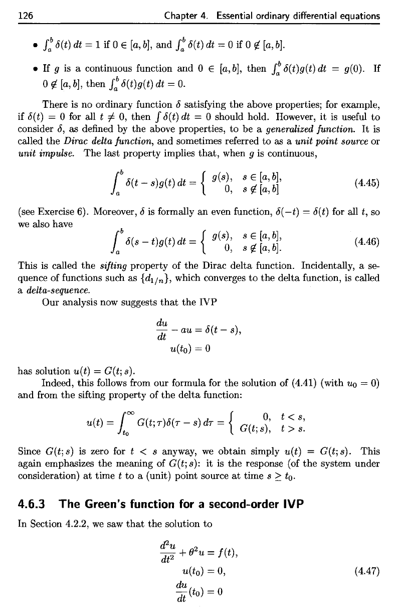
Since
G(t;
8)
is
zero for t < 8 anyway,
we
obtain simply u(t) = G(t;
8).
This
again emphasizes the meaning of
G(t; 8):
it
is
the response (of
the
system under
consideration)
at
time t to a (unit) point source
at
time s
2:
to.
4.6.3 The
Green's
function
for
a
second-order
IVP
In Section 4.2.2,
we
saw
that
the solution
to
d
2
u
dt
2
+ ()2U =
!(t),
u(to) = 0,
du
dt
(to)
= 0
( 4.47)
4.6. Green's
functions
127
4.6.4 Green's
functions
for
PDEs
We
can now
briefly
preview
the
form
of the
Green's function
for an
IVP
or
IBVP
defined
by a
PDE.
We
will assume
that
any
boundary
conditions
are
homogeneous
for
simplicity. Both
the
initial values
and the
forcing
function
will
be
prescribed over
the
spatial
domain
of the
problem,
and we
will
have
to
"add
up" the
contributions
across space
as
well
as
across time. Therefore,
the
Green's
function
will
have
the
form
G(x,
£;
£,
s),
giving
the
influence
of the
datum
at the
space-time point
(£,
s) on
the
solution
at (x, t}.
Moreover,
the
solution formula
will
involve
an
integral over
space
as
well
as
time, since
we
must
add up the
contributions across
the
spatial
domain
as
well
as
over
the
time interval.
A
similar notion
of
Green's
function
applies
in the
case
of
static
problems,
that
is,
PDEs
in
which
the
independent
variables
are
only space variables; then
G(x;
£)
defines
the
influence
of the
datum
at the
space point
£ on the
solution
at x.
This reasoning also hints
at one of the
analogies mentioned
in
Section 3.6.
The
inverse matrix
A~
l
defines
the
influence
of
each component
bj in the
data
(right-hand side)
of the
linear system
Ax.
= b on
component
Xi of the
solution:
bj
contributes
(A~
1
)ijbj
to
Xj,
and we get the
full
result
by
adding
up
over
the
position
j of the
datum component. This story
is in
precise correspondence with
the way in
which
the
Green's
function
G(£;
s)
defines
the
influence
of the
datum
at
"position" (time)
s on the
solution
at
"position"
(time)
t. So G is
presumably
in
some sense
an
inverse operator;
we
will develop
this point
of
view further
in
Chapter
5.
is
Therefore,
the
(causal) Green's
function
for
(4.47)
is
Exercises
1.
Find
the
Green's
function
for the
following
IVP:
2.
Suppose
a
certain population grows according
to the ODE
where
/ is the
immigration.
If the
population
at the
beginning
of
1990
is
55.5
million
and
immigration during
the
next
10
years
is
given
by the
function
f(t)
= 1
—
Q.2t
(in
millions), where
t = 0
represents
the
beginning
of
1990,
4.6. Green's functions
is
u(t) =
~
t sin
(O(t
-
s))f(s)
ds.
ito
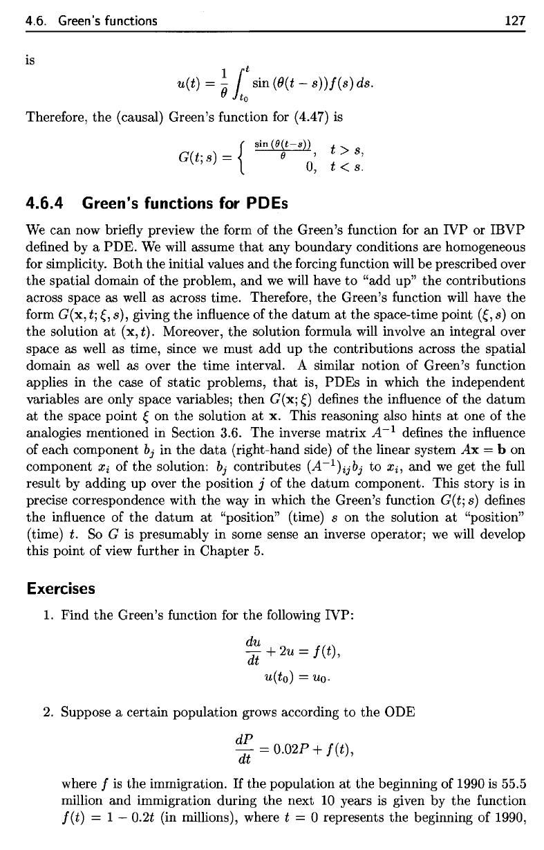
Therefore, the (causal) Green's function for (4.47)
is
{
sin
(1I(t-s))
G(t;S) =
II
0'
,
4.6.4
Green's functions for PDEs
t>
s,
t <
S.
127
We
can now briefly preview the form of
the
Green's function for
an
IVP or IBVP
defined by a PDE.
We
will assume
that
any boundary conditions are homogeneous
for simplicity. Both the initial values and the forcing function will
be
prescribed over
the
spatial domain of the problem, and
we
will have
to
"add up"
the
contributions
across space as
well
as across time. Therefore, the Green's function will have the
form G(x,
t;~,
s),
giving the influence of the
datum
at
the space-time point
(~,
s) on
the solution
at
(x, t). Moreover, the solution formula will involve
an
integral over
space as well as time, since
we
must
add
up the contributions across the spatial
domain as well as over the time interval. A similar notion of Green's function
applies in the case of static problems,
that
is, PDEs in which the independent
variables are only space variables; then
G(x;~)
defines the influence of the
datum
at
the
space point
~
on
the
solution
at
x. This reasoning also hints
at
one of
the
analogies mentioned in Section 3.6. The inverse matrix
A-I
defines the influence
of each component
b
j
in the
data
(right-hand side) of
the
linear system
Ax
= b on
component
Xi
of the solution: b
j
contributes
(A-I
)ijb
j
to
Xi,
and
we
get the full
result by adding up over the position
j of the
datum
component. This story
is
in
precise correspondence with
the
way in which
the
Green's function G(t; s) defines
the influence of the
datum
at
"position" (time) s on the solution
at
"position"
(time)
t.
So
G
is
presumably in some sense
an
inverse operator;
we
will develop
this point of view further in Chapter
5.
Exercises
1. Find
the
Green's function for
the
following IVP:
du
dt
+ 2u = f(t),
u(to) =
Uo·
2.
Suppose a certain population grows according to the ODE
dP
dt
=
0.02P
+ f(t),
where f
is
the immigration.
If
the
population
at
the beginning of 1990
is
55.5
million and immigration during the next
10
years
is
given by the function
f(t) = 1 - 0.2t (in millions), where t = 0 represents the beginning of 1990,
