Gebali F. Analysis Of Computer And Communication Networks

Подождите немного. Документ загружается.

298 8 Modeling Traffic Flow Control Protocols

8.4.2 VS Protocol Performance

Having obtained the transition matrix, we are able to calculate the performance of

the VS protocol.

The probability that an arriving cell is marked for discard is considered equal

to the cell loss probability. This happens when the source exceeds the maximum

number of penalties allowed. Thus cell loss probability is given by

L = cs

(8.80)

where c is the probability that a cell arrived while the source is nonconforming and

is the probability that the penalty queue is full.

The average number of cells that are dropped per time step is given by

(lost) = L λ

(8.81)

where λ

is the average input data rate (units cells/time step).

The efficiency or access probability p

is the probability that an arriving cell is

not dropped or marked for future discard. p

is given by

= 1 − L = 1 −cs

(8.82)

The average number of packets that are accepted without being dropped per time

step is the system throughput and is given by

Th = p

(

1 −cs

)

(8.83)

The maximum burst size allowed from the packet source is determined by the

size of the queue.

Max. burst size = B cells (8.84)

Example 8.7 Estimate the performance of the VS algorithm for a source having the

following properties:

a = 0.2 b = 0.5

c = 0.3 A = 424 bits

λ = 150 Mbps B = 5

Problems 299

The transition matrix for the VS protocol is given by

P =

⎡

⎢

⎣

0.70.20000

0.30.50.20 0 0

00.30.50.20 0

000.30.50.20

0000.30.50.2

00000.30.8

⎤

⎥

⎦

The distribution vector for the system is

s =



0.0481 0.0722 0.1083 0.1624 0.2436 0.3654



The performance figures of the protocol are as follows:

L = 0.1096

(lost) = 16.4436 ×10

packets/s

= 0.8904

Th = 133.5564 ×10

packets/s

Example 8.8 What would happen in the above example if the VS algorithm uses a

buffer whose size is B = 2?

The following table illustrates the effect of reducing the buffer size.

Parameter B = 8 B = 2

L 0.1096 0.1421

(lost) (M packets/s) 16.4436 21.3158

0.8904 0.8579

Th (M packets/s) 133.5564 128.6842

As expected, the reduced penalty buffer results in decreased performance such

as higher cell loss probability and lower throughput.

Problems

Leaky Bucket Algorithm

8.1 In a leaky bucket traffic shaper, the packet arrival rate for a certain user is

on the average 5 Mbps with a maximum burst rate of 30 Mbps. The output

rate is dictated by the algorithm to be 10 Mbps. Derive the performance of

this protocol using the M/M/1/B modeling approach assuming packet buffer

300 8 Modeling Traffic Flow Control Protocols

size to be B = 5 and the maximum line rate is 200 Mbps. Assume different

values for the probability that the source is conforming.

8.2 Repeat problem 8.1 using the M

/M/1/B modeling approach.

8.3 An alternative to modeling the leaky bucket algorithm using the M

/M/

1/B queue is to assume the Bernoulli probability of packet arrival to be

given as

a =

which is similar to the packet arrival statistics for the M/M/1/B queue. Study

this situation using the data given in Example 8.1 and comment on your re-

sults.

Token Bucket Algorithm

8.4 Consider the single arrival/departure model for the token bucket algorithm.

Assume that arriving data are buffered in a packet buffer. Now we have two

buffers to consider: the token buffer and the data buffer. Model the data buffer

based on the results obtained for the token buffer

8.5 Estimate the maximum burst size in the token bucket protocol.

8.6 In a token bucket traffic shaper, the packet arrival rate for a certain user is

on the average 15 Mbps with a maximum burst rate of 30 Mbps. Assume the

source is conforming 30% of the time and the token arrival rate is dictated

by the algorithm to be 20 Mbps. Study the state of the token buffer using

the M/M/1/B modeling approach assuming its size to be B = 5 and the

maximum line rate is 100 Mbps.

8.7 Repeat Problem 8.6 using the multiple arrival/departure modeling approach.

8.8 Draw the Markov state transition diagram for the multiple arrival/departure

model when B

= 4, B

= 3, and m = 4.

8.9 Write down the transition matrix for the above problem and compare with the

same system that had m = 3 in (8.63) on page 291.

8.10 Write down the transition matrix for the multiple arrival/departure model when

= 4, B

= 6, and m = 8.

Virtual Scheduling Algorithm

8.11 Analyze the virtual scheduling algorithm in which an arriving cell is conform-

ing if t ≥ TAT − ⌬ and is nonconforming if t < TAT − ⌬.

8.12 Compare the performance of the VS algorithm treated in the text to the VS

algorithm analyzed in Problem 8.11.

References 301

8.13 Analyze the virtual scheduling algorithm in which an arriving cell is issued a

credit or penalty according to the criteria:

credit : t ≥ TAT + ⌬

no action : TAT ≤ t < TAT +⌬

no action : ATA −⌬ ≤ t < TAT + ⌬

credit : t ≥ TAT − ⌬

References

1. A.S. Tanenbaum, Computer Networks, Prentice Hall PTR, Upper Saddle River, New Jersey,

1996.

Chapter 9

Modeling Error Control Protocols

9.1 Introduction

Modeling a protocol or a system is just like designing a digital system, or any system

for that matter — There are many ways to model a protocol based on the assump-

tions that one makes. My motivation here is simplicity and not taking a guided

tour through the maze of protocol modeling. My recommendation to the reader is

to read the discussion on each protocol and then lay down the outline of a model

that describes the protocol. The model or models developed here should then be

compared with the one attempted by the reader.

Automatic-repeat-request (ARQ) techniques are used to control transmission er-

rors caused by channel noise [1]. All ARQ techniques employ some kind of error

coding of the transmitted data so that the receiver has the ability to detect the pres-

ence of errors. When an error is detected, the receiver requests a retransmission

of the faulty data. ARQ techniques are simple to implement in hardware and they

are especially effective when there is a reliable feedback channel connecting the

receiver to the transmitter such that the round-trip delay is small.

There are three main types of ARQ techniques:

• Stop-and-wait ARQ (SW ARQ)

• Go-back-N ARQ (GBN ARQ)

• Selective-repeat ARQ (SR ARQ)

We discuss and model each of these techniques in the following sections.

9.2 Stop-and-Wait ARQ (SW ARQ) Protocol

Stop-and-wait ARQ (SW ARQ) protocol is a simple protocol for handling frame

transmission errors when the round-trip time (2τ

) for frame propagation and recep-

tion of acknowledgment is smaller than frame transmission time (τ

). The propaga-

tion delay τ

is given by

F. Gebali, Analysis of Computer and Communication Networks,

DOI: 10.1007/978-0-387-74437-7



Springer Science+Business Media, LLC 2008

303

304 9 Modeling Error Control Protocols

where c is speed of light and d is the distance between transmitter and receiver. The

transmission delay τ

is given by

where L is the number of bits in a frame and λ is the transmission rate in bits per

second.

Thus, ARQ protocols are efficient and useful when we have

2τ

 τ

(9.1)

If the above inequality is not true, then forward error correction (FEC) techniques

should be used [1].

When the sender transmits a frame on the forward channel, the receiver checks it

for errors. If there are no errors, the receiver acknowledges the correct transmission

by sending an acknowledge (ACK) signal through the feedback channel. In that

case, the transmitter proceeds to send the next frame. If there were errors in the

received frame, the receiver sends a negative acknowledgment signal (NAK) and

the sender sends the same frame again. If the receiver does not receive ACK or

NAK signals due to some problem in the feedback channel, the receiver waits for a

certain timeout period and sends the frame again.

Based on the above discussion, we conclude that the time between transmitted

frames is equal to 2τ

, where τ

is the one-way propagation delay.

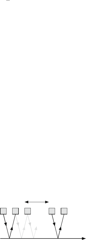
Figure 9.1 shows an example of transmitting several frames using stop-and-wait

ARQ. Frame 1 was correctly received as indicated by the ACK signal and the sender

starts sending frame 2.

Frame 2 was received in error as indicated by NAK and the grey line. The trans-

mitter sends frame 2 one more time. For some reason, no acknowledgment signals

were received (indicated by short grey line) and the sender sends frame 2 for the

third time after waiting for the proper timeout period.

Frame 2 was received correctly as indicated by the ACK signal and the sender

starts sending frame 3.

Fig. 9.1 Stop-and-wait ARQ

protocol

...

1 2 2 2

Time-out period

ACK

Receiver

Transmitter

Channel

NAK

ACK

Lost

Time

9.2 Stop-and-Wait ARQ (SW ARQ) Protocol 305

9.2.1 Modeling Stop-and-Wait ARQ

In this section, we perform Markov chain analysis of the stop-and-wait algorithm.

We make the following assumptions for our analysis of the stop-and-wait ARQ

(SW ARQ):

1. The average length of a frame is n bits.

2. The forward channel has random noise and the probability that a bit will be

received in error is . Another name for  is bit error rate (BER) .

3. The feedback channel is assumed noise-free so that acknowledgment signals

from the receiving station will always be transmitted to the sending station.

4. The sender will keep sending a frame until it is correctly received. The effect of

limiting the number of retransmissions is discussed in Problem 9.2.

The state of the sender while attempting to transmit a frame depends only on the

outcome of the frame just sent. Hence we can represent the state of the sender as a

Markov chain having the following properties:

1. State i of the Markov chain indicates that the sender is retransmitting the frame

for the ith time. State 0 indicates error-free transmission.

2. The number of states is infinite since no upper bound is placed on the number of

retransmissions.

3. The time step is taken equal to the sum of transmission delay and round-trip

delay T = τ

+2τ

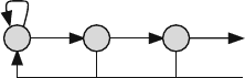
The state transition diagram for the SW ARQ protocol is shown in Fig. 9.2. In

the figure, e represents the probability that the transmitted frame contained an error.

e is given by the expression

e = 1 −(1 −)

(9.2)

For a noise-free channel  = 0 and so e = 0. When the average number of errors

in a frame is very small (i.e.,  n  1), we can write

e ≈  n (9.3)

The quantity  n is an approximation of the average number of bits in error in a

frame (see Problems 9.4 and 9.5). Naturally, we would like the number of errors to

be small so as not to waste the bandwidth in retransmissions. Thus, we must have

e =  n  1 (9.4)

Fig. 9.2 State transition

diagram of a sending station

using the SW ARQ error

control protocol

...

1-e

eee

1-e

306 9 Modeling Error Control Protocols

Equation (9.2) assumed no forward error correction (FEC) coding is imple-

mented. Problem 9.4 requires you to derive an expression for e when FEC is

employed.

We organize the state distribution vector as follows:

s =



···



(9.5)

where s

corresponds to retransmitting the frame for the ith time. s

corresponds

to transmitting the frame once with zero retransmissions. This is the case when the

frame was correctly received without having to retransmit it.

The corresponding transition matrix of the channel is given by

P =

⎡

⎢

⎣

1 −e 1 −e 1 −e 1 −e ···

e 000···

0 e 00···

00e 0 ···

⎤

⎥

⎦

(9.6)

At equilibrium, the distribution vector is obtained by solving the two equations

Ps= s (9.7)



s = 1 (9.8)

The solution to the above two equations is simple:

s = (1 −e) ×



1 ee

···



(9.9)

9.2.2 SW ARQ Performance

The average number of retransmissions for a frame is given by

= (1 −e) ×

(

+2s

+3s

+···

)

= (1 −e)

∞



i=0

= e transmissions/frame (9.10)

For a noise-free channel, e = 0 and the average number of retransmissions is

also 0. This indicates that a frame is sent once for a successful transmission.

For a typical channel, e ≈  n  1 and the average number of transmissions can

be approximated as

≈  n (9.11)

9.2 Stop-and-Wait ARQ (SW ARQ) Protocol 307

We define the efficiency of the SW ARQ protocol as the inverse of the total num-

ber of transmissions which includes the first transmission plus the average number

of retransmissions. In that case, η is given by

η =

1 + N

1 +e

(9.12)

For an error-free channel, N

= 0 and η = 100%. For a typical channel,

e ≈  n  1 and the efficiency is given by

η ≈ 1 − n (9.13)

This indicates that the efficiency decreases with increase in bit error rate or frame

size. Thus, we see that the system performance will degrade gradually with any

increase in the number of bits in the frame or any increase in the frame error proba-

bility.

The throughput of the transmitter can be expressed as

Th = η = 1 −e frames/time step (9.14)

Thus, for an error-free channel, η = 1 and arriving frames are guaranteed to be

transmitted on the first try. We could have obtained the above expression for the

throughput by estimating the number of frames that are successfully transmitted in

each transmitter state:

Th = (1 −e)

∞



i=0

= 1 −e (9.15)

When errors are present in the channel, then η<1 and so is the system

throughput.

Example 9.1 Assume an SW ARQ protocol in which the frame size is n = 1000

and the bit error rate is  = 10

−4

. Find the performance of the SW ARQ protocol for

this channel. Repeat the example when the bit error rate increases by a factor of 10.

According to (9.10), the average number of transmissions for a window is

= 0.1052

and the efficiency is

η = 90.48%

Notice that because the bit error rate is low, we need just about one transmission

to correctly receive a frame.

308 9 Modeling Error Control Protocols

Now we increase the bit error rate to e = 10

−3

and get the following results.

= 1.7196

and the efficiency is

η = 36.77

Notice that when the bit error rate is increased by one order of magnitude, the

average number of frame retransmission is increased by a factor of 16.35.

9.3 Go-Back-N (GBN ARQ) Protocol

In the go-back-N protocol, the transmitter keeps sending frames but keeps a copy

in a buffer, which is called the transmission window. The number of frames in the

buffer, or the window, is N which equals the number of frames sent during one

round-trip time.

When the sender transmits the frames on the forward channel, the receiver checks

them for errors. If there are no errors, the receiver acknowledges each frame by

sending acknowledge (ACK) signals through the feedback channel. Upon reception

of an ACK for a certain frame, the receiver drops it from the head of its buffer. If

a received frame is in error, the receiver sends a negative acknowledgment signal

(NAK) for that particular frame. When the transmitter receives the NAK signal, it

resends all N frames in its buffer starting with the frame in error.

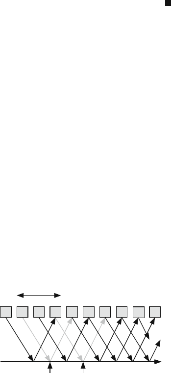
Figure 9.3 shows an example of transmitting several frames using go-back-N

where the buffer size is N = 3. Solid arrows indicate ACK signals and grey arrows

indicate NAK signals. Frame 1 was correctly received while frame 2 was received

in error. We see that the transmitter starts to send frame 2 and the three subsequent

frames that were in its buffer.

Fig. 9.3 Go-back-N ARQ

protocol with buffer size

N = 3. Solid arrows indicate

ACK signals and grey arrows

indicate NAK signals

...

1 2

Window Size

Receiver

Transmitter

Channel

Time

3 4

3 4 5 4

Error Error