Gebali F. Analysis Of Computer And Communication Networks
Подождите немного. Документ загружается.

288 8 Modeling Traffic Flow Control Protocols
L = 0.7453
Th = 0.1482 packets/time step
Th
=3.7051 × 10
4
packets/s
p
a
=0.57
Q
a
= 2.1533 packets
W = 14.5294 times steps
W
=5.8118 × 10
−5
s
Example 8.4 Investigate the effect of doubling the token buffer or the packet buffer
on the performance of the token bucket algorithm in the above example.
Doubling the token buffer to B
t
= 4 or doubling the packet buffer result in the
following parameters:
Parameter B
t
= 2, B
p
= 3 B
t
= 4, B
p
= 3 B
t
= 2, B
p
= 6
N
a
(lost) 0.1118 0.1104 0.1102
L 0.4300 0.4248 0.4239
Th 0.1482 0.1496 0.1498
p
a
0.57 0.5752 0.5761
Q
a
2.1533 2.1274 5.0173
W 14.5294 14.2250 33.4988
We note that increasing the buffer size improves the system performance. How-
ever, doubling the packet buffer size doubles the delay without too much improve-
ment in throughput compared to doubling the token buffer size.
8.3.4 Multiple Arrivals/Single Departures Model (M
m
/M /1/B)
In this approach to modeling the token bucket algorithm, we take the time step equal
to the inverse of the fixed token arrival rate.
T =
1
λ
t
(8.54)
where T is measured in units of seconds and λ
t
is the token arrival rate in units
of packets/s. Usually, λ
l
is specified in units of bits per second. In that case, T is
obtained as
T =
A
λ
t
(8.55)
where A is the average packet length.
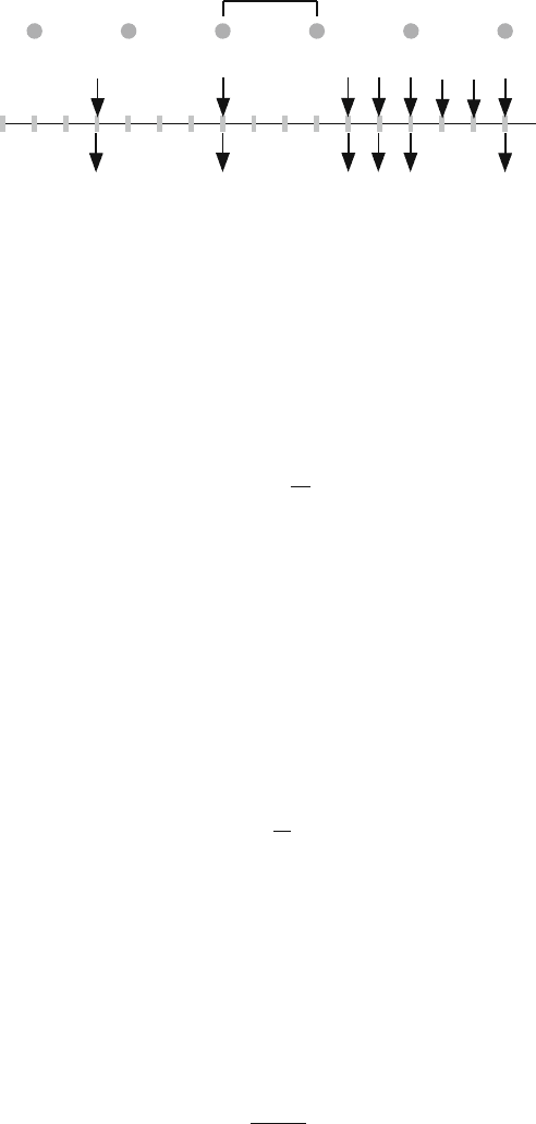
Figure 8.9 shows the events of packet arrival and departure and also the time step
value as indicated by the spacing between the successive tokens.
Thus at a given time step only one token arrives at the buffer and one or more
tokens can leave if the buffer is not empty and data arrives. The token arrival prob-
ability per time step is given by
8.3 The Token Bucket Algorithm 289
time step
Output traffic with
variable rate
4
4
5
5
time
12
2
3
3
6
7
1
Input traffic with
variable rate
Arriving token
at fixed rate
6
8
Fig. 8.9 Events of packet arrival and departure for the token bucket algorithm. The time step value
is equal to the time between two adjacent arriving tokens
a = 1 (8.56)
The average number of arriving packets per time step is given by
N
a
(in) =
λ
a
λ
t
(8.57)
where the average input data rate (λ
a
) is given as before by
λ
a
= pλ
a
+(1 − p)σ (8.58)
where p is the probability that the source is producing data at the rate λ
a
and 1 − p
is the probability that the source is producing data at the burst rate σ . λ
a
could be
smaller or larger than λ
t
depending on the probability p.
The maximum number of packets (N) that could arrive at the queue input as
determined by the burst rate σ
N =
$
σ
λ
t
%
(8.59)
with x is the smallest integer that is larger than or equal to x. The average number
of packets that arrive per time step is given from (8.57) and (8.59) according to the
binomial distribution as
Nx= N
a
(in) (8.60)
where x is the probability of a packet arriving. The above equation gives x as
x =
N
a
(in)
N
(8.61)
290 8 Modeling Traffic Flow Control Protocols
Thus we are now able to determine the packet arrival probabilities as
c
i
=
N
i
x
i
(1 − x)
L−i
i = 0, 1, 2, ..., N (8.62)
The state of occupancy of the token buffer depends on the statistics of token and
packet arrivals as follows:
1. The token buffer will stay at the same state with probability c
1
, i.e., when one
packet arrives.
2. The token buffer will increase in size by one with probability c
0
; i.e., when no
packets arrive.
3. The token buffer will decrease in size by one with probability c
2
; i.e., when two
packets arrive.
4. The token buffer will decrease in size by i with probability c
i+1
; i.e., when i +1
packets arrive with i < N
The state of occupancy of the packet buffer depends on the statistics of token and
packet arrivals as follows
1. The packet buffer will stay at the same state with probability c
1
, i.e., when one
packet arrives.
2. The packet buffer will decrease in size by one with probability c
0
; i.e., when no
packets arrive.
3. The packet buffer will increase in size by one with probability c
2
; i.e., when two
packets arrive.
4. The packet buffer will increase in size by i with probability c
i+1
; i.e., when i +1
packets arrive with i < N
Based on the above discussion, we have two buffers to hold the tokens and the
packets. The token buffer is single-input multiple output while the packet queue is
multiple input, single-output. The size of the token buffer is assumed B
t
and the size
of the packet buffer is assumed B
p
.
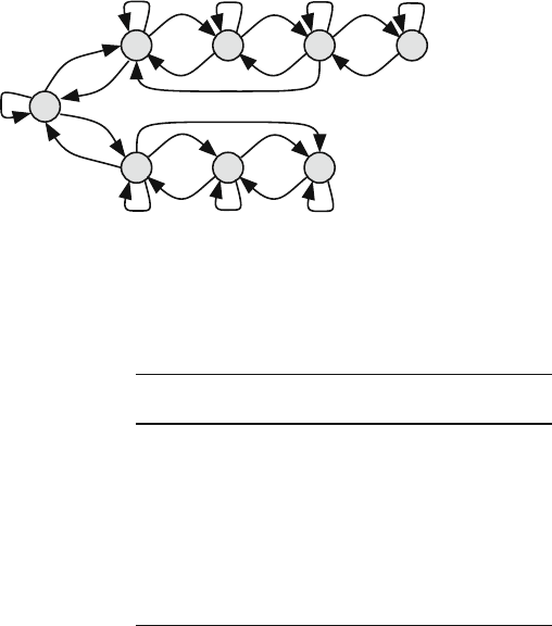
Figure 8.10 shows the Markov chain transition diagram for the system compris-
ing the token and packet buffers. The upper row represents the states of the token
buffer and the lower row represents the states of the packet buffer. The transition
probabilities are dictated by the packet arrival probabilities and the states of occu-
pancy of the token and packet buffers. The figure shows a token buffer whose size is
B
t
= 4 and a packet buffer whose size is B
p
= 3. The maximum number of packets
that could arrive in one time step is assumed N = 3. Figure 8.10 shows the c
0
, c
1
,
and c
2
transitions. The c
3
transitions are only shown out of states s
4
and s
6
in order
to reduce the clutter.
The meaning of each state is shown in Table 8.2.
The transition matrix of the composite system is a
B
t
+ B
p
+1
×
B
t
+ B
p
+1
tridiagonal matrix. For the case when B
t
= 4, B
p
= 3, and, N = 3, the matrix is
given by
8.3 The Token Bucket Algorithm 291
P =
⎡
⎢
⎢
⎢
⎢
⎢
⎢
⎢
⎢
⎢
⎢
⎢
⎢
⎣
c
1
c
2
c
3
00 c
0
00
c
0
c
1
c
2
00 0 0 0
0 c
0
c
1
c
2
0000
00c
0
c
1
c
2
00 0
000c
0
1 −c
2
00 0
c
2
c
3
00 0 c
1
c
0
0
c
3
000 0 c
2
c
1
c
0
0000 0 c
3
c
2
+c
3
1 −c
0
⎤
⎥
⎥
⎥
⎥
⎥
⎥
⎥
⎥
⎥
⎥
⎥
⎥
⎦
(8.63)
8.3.5 Token Bucket Performance (Multiple Arrival/Departure
Case)
Having obtained the transition matrix, we are able to calculate the performance
figures of the token bucket protocol.
The throughput of the token bucket algorithm is the average number of packets
per time step that are produced without being tagged or lost. To find the throughput
N
s
2
s
3
s
4
s
5
c
0
c
1
s
1
s
6
s
7
s
8
c
2
c
3
c
2
c
2
c
2
c
0
c
1
c
1
c
1
c
0
c
0
c
2
c
2
c
2
c
3
c
0
c
1
c
0
c
1
c
0
1-c
0
1-c
2
Token buffer states
Packet buffer states
Fig. 8.10 Markov chain transition diagram for the system comprising the token and packet buffers.
Token buffer size is B
t
= 4, packet buffer size is B
p
= 3, and N = 3. The c
3
transitions are only
shown out of states s
4
and s
6
in order to reduce the clutter
Table 8.2 Defining the
binomial coefficient
Token buffery Packet buffer
State occupancy occupancy
s
1
00
s
2
10
s
3
20
s
4
30
s
5
40
s
6
01
s
7
02
s
8
03
292 8 Modeling Traffic Flow Control Protocols
we must study all the states of the combined system. It is much easier to obtain the
throughput using the traffic conservation principle after we find the lost traffic.
Packets are lost or tagged for future discard if more than one packet arrives when
the packet buffer cannot accommodate all of them.
When N < B
p
, the average number of lost or tagged packets per time step is
given by
N
a
(lost) =
B
p
−1
i=1
s
B
t
+B
p
+2−i
N
j=i+1
i ( j − 1)c
j
(8.64)
The lost traffic is measured in units of packets/time step. And the number of
packets lost per second is
N
a
(lost) =
N
a
(lost)
T
= N
a
(lost) λ
l
(8.65)
The average number of packets arriving per time step is given by
N
a
(in) =
N
i=0
ic
i
= Nx (8.66)
The packet loss probability is
L =
N
a
(lost)
N
a
(in)
=
N
a
(lost)
Nc
(8.67)
The throughput of the token bucket algorithm is obtained using the traffic con-
servation principle
Th = N
a
(in) − N
a
(lost)
= Nc− N
a
(lost) (8.68)
The throughput is measured in units of packets/time step. The throughput in units
of packets/second is expressed as
Th
=
Th
T
= Th ×λ
l
(8.69)
The packet acceptance probability of the token bucket algorithm is
p
a
=
Th
N
a
(in)
=1 −
N
a
(lost)
Nc
(8.70)

8.3 The Token Bucket Algorithm 293
We remind the reader that packet acceptance probability is just another name for
the efficiency of the token bucket algorithm. It merely indicates the percentage of
packets that make it through that traffic regulator without getting lost or tagged.
The average queue size for the tokens is given by
Q
t
=
B
t
i=1
is
i+1
(8.71)
Notice the value of the state index in the above equation.
The average queue size for the packets is given by
Q
p
=
B
p
i=1
is
i+B
t
+1
(8.72)
Notice the value of the state index in the above equation.
Using Little’s result, the average wait time or delay for the packets in the packet
buffer is
W =
Q
p
Th
(8.73)
The wait time is measured in units of time steps. The wait time in seconds is
given by
W
=
Q
p
Th
(8.74)
Example 8.5 Repeat Example 8.3 using the multiple arrival/departure modeling
approach.
The maximum number of packets that could arrive in one time step m is found
as
N =
$
σ
λ
out
%
= 4
The average input data rate is
λ
a
= 10 ×0.6 +50 ×0.4 = 26 Mbps
The packet arrival probability is
x =
26
100
= 0.4333
The probability that k packets arrive in one time step is

294 8 Modeling Traffic Flow Control Protocols
c
k
=
4
k
a
k
b
4−k
k = 0, 1, 2
The transition matrix will be 6 ×6 and is given by
P =
⎡
⎢
⎢
⎢
⎢
⎢
⎢
⎣
0.3154 0.3618 0.1844 0.1031 0 0
0.1031 0.3154 0.3618 0 0 0
00.1031 0.4184 0 0 0
0.3618 0.1844 0.0353 0.3154 0.1031 0
0.1844 0.0353 0 0.3618 0.3154 0.1031
0.0353 0 0 0.2197 0.5815 0.8965
⎤
⎥
⎥
⎥
⎥
⎥
⎥
⎦
The equilibrium distribution vector is
s =
0.0039 0.0006 0.0001 0.0231 0.1388 0.8334
t
State s
2
indicates that there is a 0.0006 probability that there is one token in
the token buffer. State s
6
indicates that 83.34% of the time the packet buffer is full
indicating the source is misbehaving and the packet buffer is full.
The throughput of the queue is given by
N
a
(lost) = 0.3279 packets/time step
N
a
(lost) = 1.2298 ×10
4
packets/s
L = 0.1892
Th = 1.4054 packets/time step
Th
=5.2702 ×10
4
packets/s
p
a
= 0.8108
Q
a
= 2.8 packets
W = 1.9931 time steps
W
=5.3149 ×10
−5
s
Example 8.6 Investigate the effect of doubling the token buffer or the packet buffer
on the performance of the token bucket algorithm in the above example.
Doubling the token buffer to B
t
= 4 or doubling the packet buffer result in the
following parameters:
Parameter B
t
= 2,B
p
= 3 B
t
= 4, B
p
= 3 B
t
= 2, B
p
= 6
N
a
(lost) 0.3279 0.3279 0.3279
L 0.1892 0.1892 0.1892
Th 1.4054 1.4054 1.4054
p
a
0.8108 0.8108 0.8108
Q
a
2.8011 2.8011 5.8002
W 1.9931 1.9931 4.1271

8.4 Virtual Scheduling (VS) Algorithm 295
Because the token buffer was nearly empty in the original system, doubling the
size of the token buffer has no impact on the system performance as can be seen
by comparing the second and third columns of the above table. Doubling the packet
buffer size doubles the delay without noticeable improvement in throughput.
8.4 Virtual Scheduling (VS) Algorithm
The virtual scheduling (VS) algorithm manages the ATM network traffic by closely
monitoring the cell arrival rate. When a cell arrives, the algorithm calculates the
theoretical arrival time (TAT) of the next cell according to the formula
TAT =
1
λ
a
(8.75)
where λ
a
is the expected average data rate (units of cells/second). TAT is measured
by finding the difference between the arrival times of the headers of two consecutive
ATM cells as explained in Fig. 8.11. This is not the time between the last bit of one
cell and the first bit of the other.
If the cell arrival rate is in units of bits/second, then TAT is written as
TAT =
A
λ
a
(8.76)
where A is the size of an ATM cell which is 424 bits.
Assuming the time difference between the current cell and the next cell is t, then
the cell is treated as conforming if t satisfies the following inequality
t ≥ TAT − ⌬ (8.77)
time
Interarrival time
Cell n Cell n + 1
Fig. 8.11 Measuring the interarrival time between two consecutive ATM cells

296 8 Modeling Traffic Flow Control Protocols
where ⌬ is a small time value to allow for the slight variations in the data rate. The
cell is treated as misbehaving, or nonconforming, when the cell arrival time satisfies
the inequality
t < TAT − ⌬ (8.78)
The problem with the above two equations is that a source could keep sending
data at a rate slightly higher than λ
a
and still be conforming if every cell arrives
within the bound of (8.77).
Figure 8.12 shows the different cases for cell arrival in VS. Figure 8.12(a) shows
a conforming cell because the cell arrival time satisfies (8.77). Figure 8.12(b) shows
another conforming cell because the arrival time still satisfies (8.77). Figure 8.12(c)
also shows a conforming cell because the arrival time satisfies the equality part of
(8.77). Figure 8.12(d) shows a nonconforming cell because the arrival time does not
satisfy (8.77).
8.4.1 Modeling the VS Algorithm
In this section, we perform Markov chain analysis of the virtual scheduling algo-
rithm. We make the following assumptions for our analysis of the virtual scheduling
algorithm.
1. The states of the Markov chain represent how many times the arriving cells from
a certain flow have been nonconforming. In other words, state s
i
of the penalty
queue indicates that the source has been nonconforming i times.
time
current cell event
TAT
Δ
time
next cell event
time
time
next cell event
next cell event
next cell event
(a)
(b)
(c)
(d)
Fig. 8.12 Different cases for cell arrival in the VS algorithm. (a) t > TAT and cell is conforming.
(b) t = TAT and cell is conforming. (c) t = TAT −⌬ and cell is conforming. (d) t < TAT −⌬ and
cell is nonconforming
8.4 Virtual Scheduling (VS) Algorithm 297
2. The number of states (B) of the queue will dictate the maximum burst size tol-
erated. Which is equal to the maximum number of penalties allowed for that
source.
3. The queue changes states upon arrival of each cell.
4. Credit is given to the source each time it is conforming.
5. A penalty is given to the source each time it is nonconforming.
6. a is the probability that the arriving cell satisfies the inequality t ≥ TAT. In that
case, credit is issued to the source.
7. b is the probability that the arriving cell satisfies the following inequality
TAT − ⌬ ≤ t ≤ TAT
In that case, no credit or penalty is issued.
8. c is the probability that the arriving cell satisfies the inequality t < TAT. In that
case, a penalty is issued to the source.
Of course, c = 1 −a −b since the source cannot be in any other state.
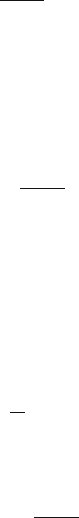
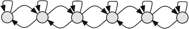
Based on the above assumptions, we have a single arrival, single departure
M/M/1/B queue with B + 1 states. Figure 8.13 shows the state transitions for
the VS queue.
It is interesting to note that the state transition diagram of the virtual scheduling
algorithm in Fig. 8.13 is a special case of the state transition diagram for the token
bucket algorithm in Fig. 8.8 when the token bucket buffer size is B
t
= 1.
The corresponding transition matrix P will be (B + 1) × (B + 1) and will have
the following entries for the case B = 5.
P =
⎡
⎢
⎢
⎢
⎢
⎢
⎢
⎣
1 −ca000 0
cba00 0
0 cba00
00cba 0
000cb a
0000c 1 −a
⎤
⎥
⎥
⎥
⎥
⎥
⎥
⎦
(8.79)
Notice that the transition matrix is tridiagonal because of the single arrival, single
departure feature of the queue.
0
2
3
4
5
aaaa
cccc
1
-
c bbb1
-
a
1
a
c
b
Fig. 8.13 State transition diagram for the VS queue for the case B = 5