Farin G. Curves and Surfaces for CAGD. A Practical Guide
Подождите немного. Документ загружается.

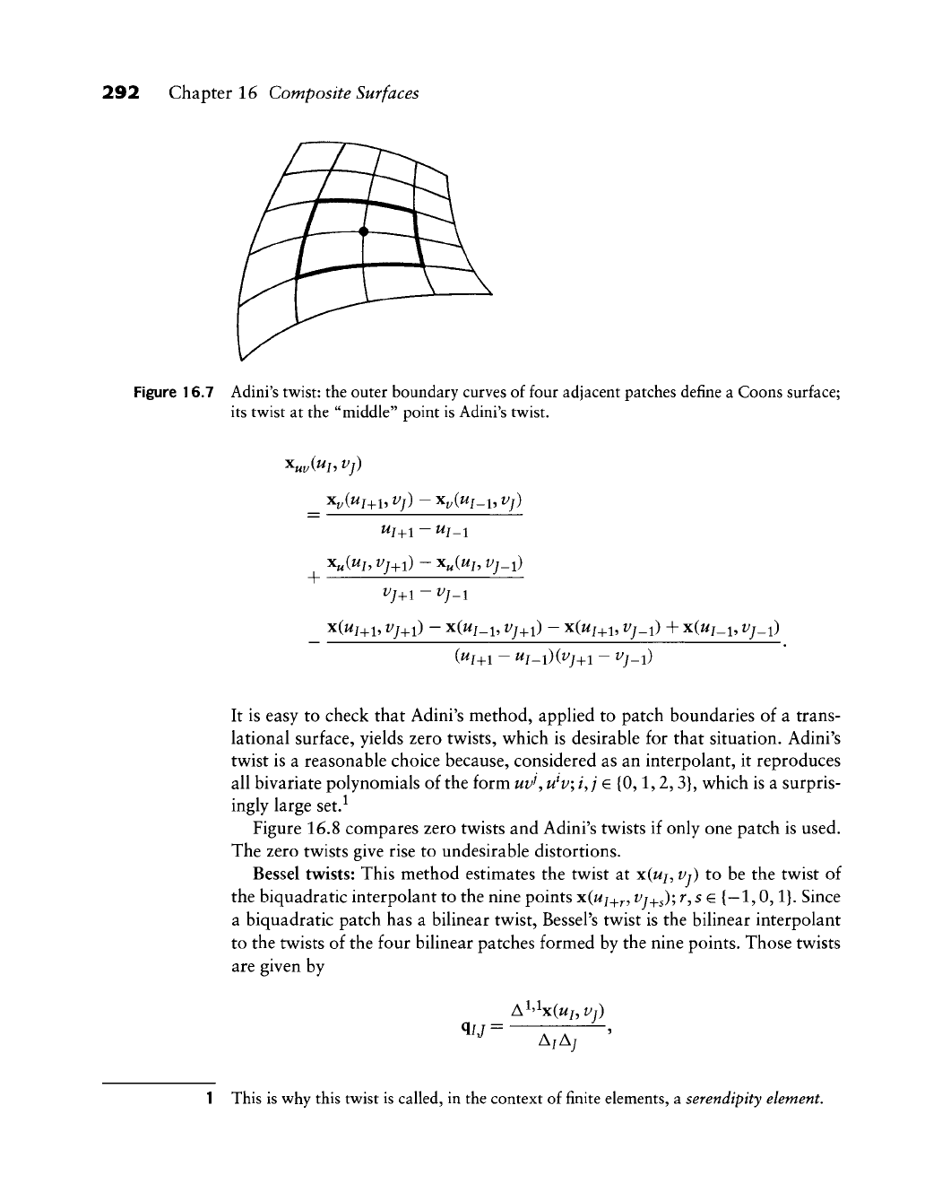
292 Chapter 16 Composite Surfaces
Figure 16.7 Adini's twist: the outer boundary curves of four adjacent patches define a Coons surface;
its twist at the "middle" point is Adini's twist.
+
Uj_^l
- Uj_i
X(^j^l, Vj^l) - x{Uj_i, Vj^i) - XJUj^i, Vj_i) + X(Uj_i, Vj_i)
It is easy to check that Adini's method, apphed to patch boundaries of a trans-
lational surface, yields zero twists, which is desirable for that situation. Adini's
twist is a reasonable choice because, considered as an interpolant, it reproduces
all bivariate polynomials of the form uv^,
u^v;
ij e
{0,1,2,3},
which is a surpris-
ingly large set.^
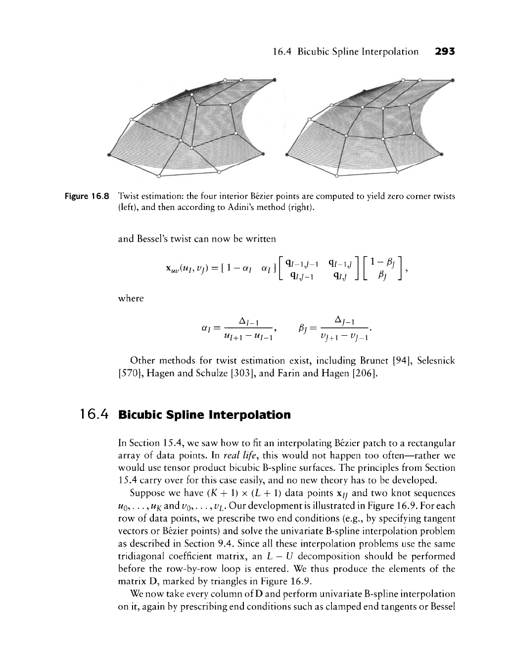
Figure 16.8 compares zero twists and Adini's twists if only one patch is used.
The zero twists give rise to undesirable distortions.
Bessel twists: This method estimates the twist at x(wj, Vj) to be the twist of
the biquadratic interpolant to the nine points
x(wj_^^,
^'^+5);
r, s € {—1,0,1}. Since
a biquadratic patch has a bilinear twist, Bessel's twist is the bilinear interpolant
to the twists of the four bilinear patches formed by the nine points. Those twists
are given by
q/j =
A^'^x(ui,Vj)
A/A;
1 This is why this twist is called, in the context of finite elements, a
serendipity
element.
16.4 Bicubic Spline Interpolation 293
Figure 16.8 Twist estimation: the four interior Bezier points are computed to yield zero corner twists
(left),
and then according to Adini's method (right).
and Bessel's twist can now be written
^uvi^h vj) = [l-ai aj]
where
Q/-i,/-i
Q/-1,/
q/,/-i
q/j
ai =
^i-i
Uj_^l - Ui_i
Pj =
V-i
^/+i ~ ^/-l
Other methods for twist estimation exist, including Brunet [94], Selesnick
[570],
Hagen and Schulze
[303],
and Farin and Hagen
[206].
1
6.4 Bicubic Spline Interpolation
In Section 15.4, we saw how to fit an interpolating Bezier patch to a rectangular
array of data points. In real life^ this would not happen too often—rather we
would use tensor product bicubic B-spline surfaces. The principles from Section
15.4 carry over for this case easily, and no new theory has to be developed.
Suppose we have (K + 1) x (L + 1) data points X/y and two knot sequences
WQ,
.
. .,
/^l^
and
i/Q,.
. ., Vi. Our development is illustrated in Figure 16.9. For each
row of data points, we prescribe two end conditions (e.g., by specifying tangent
vectors or Bezier points) and solve the univariate B-spline interpolation problem
as described in Section 9.4. Since all these interpolation problems use the same
tridiagonal coefficient matrix, an L
—
17 decomposition should be performed
before the row-by-row loop is entered. We thus produce the elements of the
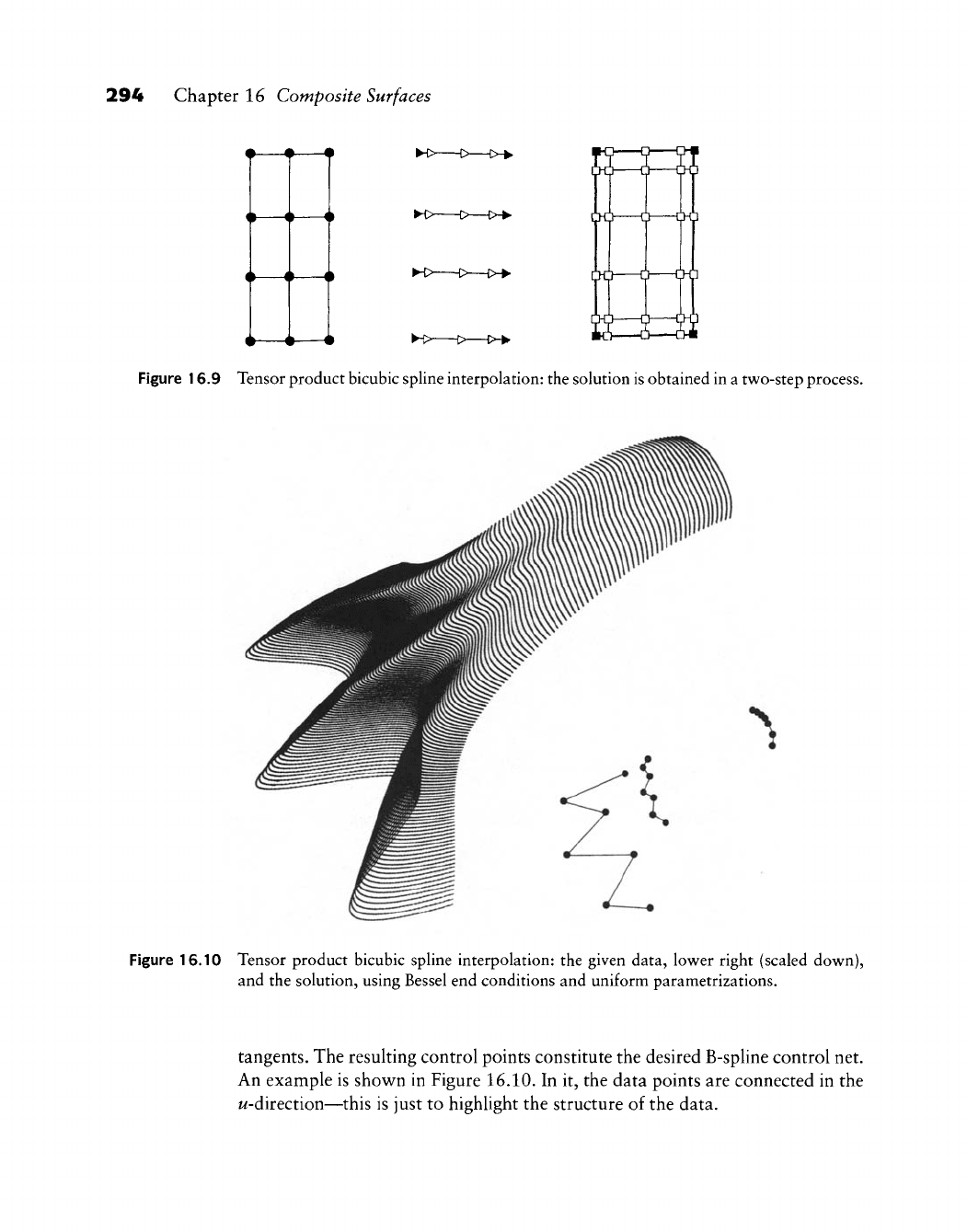
matrix D, marked by triangles in Figure 16.9.
We now take every column of D and perform univariate B-spline interpolation
on it, again by prescribing end conditions such as clamped end tangents or Bessel
294 Chapter 16 Composite Surfaces
T—T—T
T—T—7
T—T—T
i—4—i
Q
D
Figure 16.9 Tensor product bicubic spline interpolation: the solution
is
obtained in a two-step process.
^
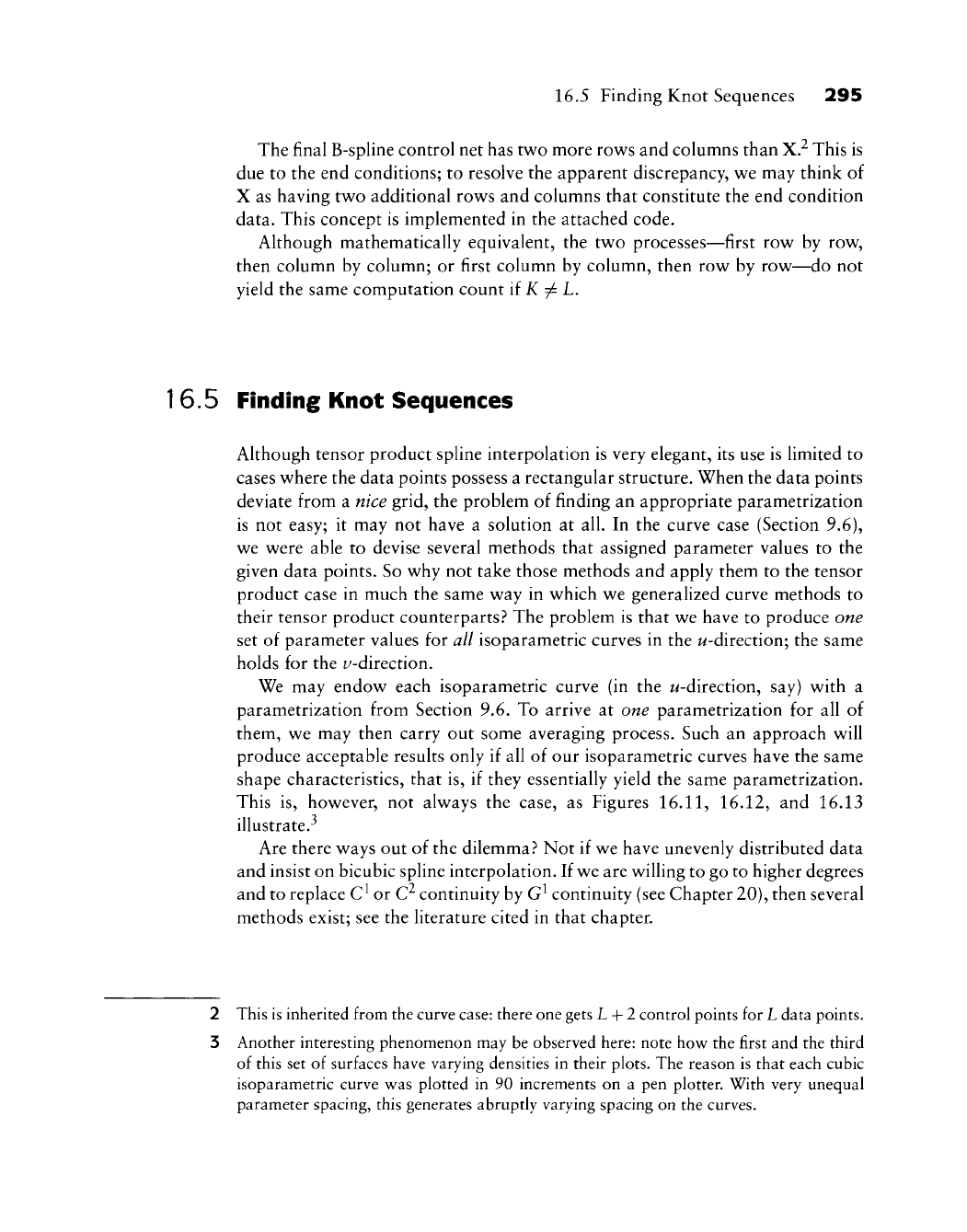
Figure 16.10 Tensor product bicubic spline interpolation: the given data, lower right (scaled down),
and the solution, using Bessel end conditions and uniform parametrizations.
tangents. The resulting control points constitute the desired B-spline control net.
An example is shown in Figure 16.10. In it, the data points are connected in the
w-direction—this is just to highlight the structure of the data.
16.5 Finding Knot Sequences 295
The final B-spline control net has two more rows and columns than X.^ This is
due to the end conditions; to resolve the apparent discrepancy, we may think of
X as having two additional rows and columns that constitute the end condition
data. This concept is implemented in the attached code.
Although mathematically equivalent, the two processes—first row by row,
then column by column; or first column by column, then row by row—do not
yield the same computation count if K
7^
L.
1
6.5 Finding Knot Sequences
Although tensor product spline interpolation is very elegant, its use is limited to
cases where the data points possess a rectangular structure. When the data points
deviate from a nice grid, the problem of finding an appropriate parametrization
is not easy; it may not have a solution at all. In the curve case (Section 9.6),
we were able to devise several methods that assigned parameter values to the
given data points. So why not take those methods and apply them to the tensor
product case in much the same way in which we generalized curve methods to
their tensor product counterparts.^ The problem is that we have to produce one
set of parameter values for all isoparametric curves in the ^-direction; the same
holds for the z/-direction.
We may endow each isoparametric curve (in the ^-direction, say) with a
parametrization from Section 9.6. To arrive at one parametrization for all of
them, we may then carry out some averaging process. Such an approach will
produce acceptable results only if all of our isoparametric curves have the same
shape characteristics, that is, if they essentially yield the same parametrization.
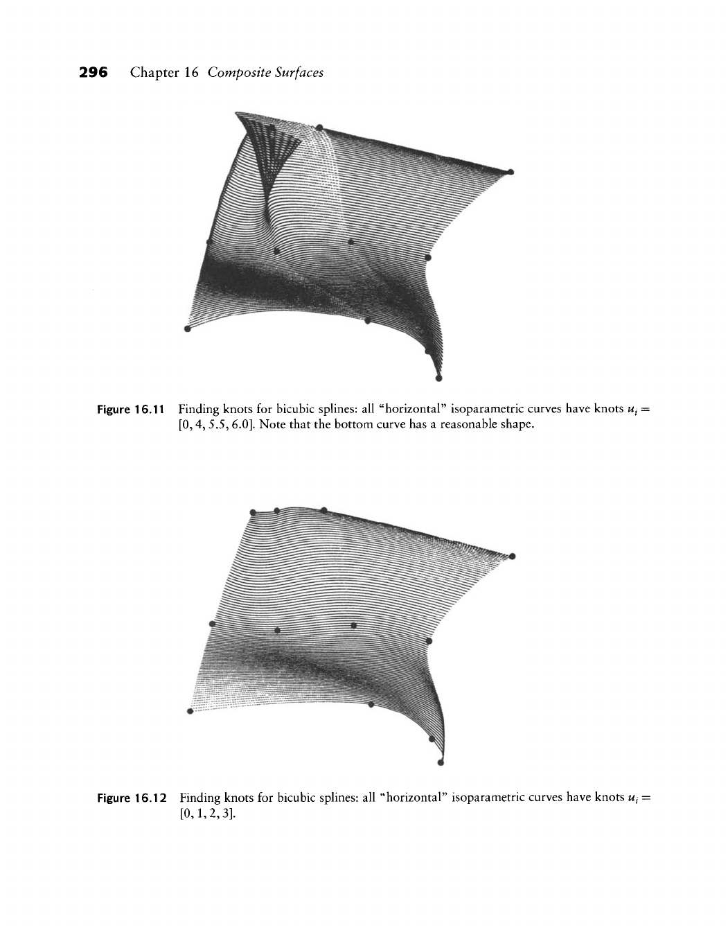
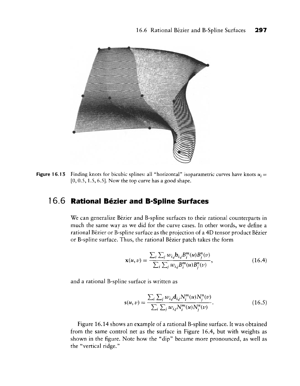
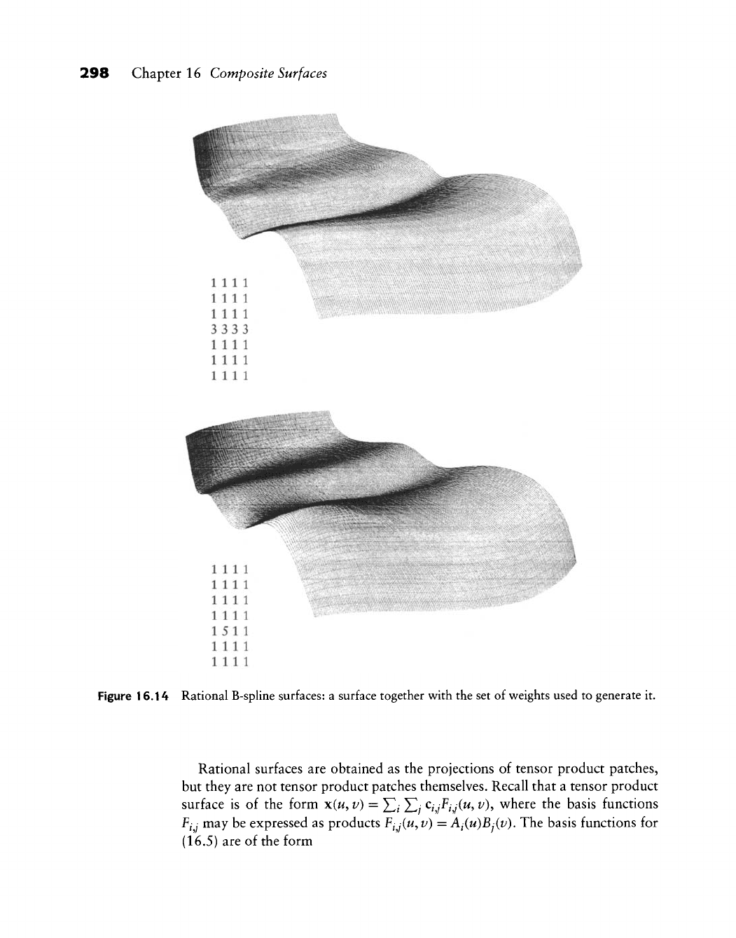
This is, however, not always the case, as Figures
16.11,
16.12, and 16.13
illustrate.^
Are there ways out of the dilemma.^ Not if we have unevenly distributed data
and insist on bicubic spline interpolation. If we are willing to go to higher degrees
and to replace C^ or C^ continuity by G^ continuity (see Chapter 20), then several
methods exist; see the literature cited in that chapter.
2 This is inherited from the curve
case:
there one gets L + 2 control points for
L
data points.
3 Another interesting phenomenon may be observed here: note how the first and the third
of this set of surfaces have varying densities in their plots. The reason is that each cubic
isoparametric curve was plotted in 90 increments on a pen plotter. With very unequal
parameter spacing, this generates abruptly varying spacing on the curves.
296 Chapter 16 Composite Surfaces
Figure 16.11 Finding knots for bicubic splines: all "horizontal" isoparametric curves have knots
Ui •
[0,4,
S.S^ 6.0]. Note that the bottom curve has a reasonable shape.
Figure 16.12 Finding knots for bicubic sphnes: all "horizontal" isoparametric curves have knots
Ui ••
[0,1,2,3].
16.6 Rational Bezier and B-Spline Surfaces 297
Figure
16.1
3 Finding knots for bicubic splines: all "horizontal" isoparametric curves have knots ui =
[0,
0.5,1.5,
6.5].
Novv^
the top curve has a good shape.
16.6 Rational Bezier and B-Spiine Surfaces
We can generalize Bezier and B-spline surfaces to their rational counterparts in
much the same way as we did for the curve cases. In other words, we define a
rational Bezier or B-spline surface as the projection of a 4D tensor product Bezier
or B-spline surface. Thus, the rational Bezier patch takes the form
x(w, v) =
(16.4)
and a rational B-spline surface is written as
E,E;^,,A,N,"'(^)N;(t/)
E,E;^,vNr(«)N;(i^) •
s(w, v) =
(16.5)
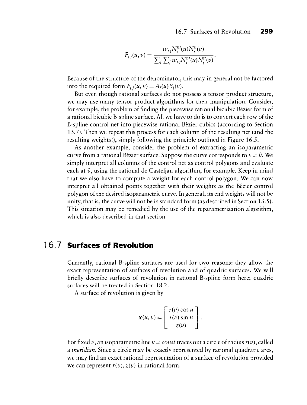
Figure 16.14 shows an example of a rational B-spline surface. It was obtained
from the same control net as the surface in Figure 16.4, but with weights as
shown in the figure. Note how the "dip" became more pronounced, as well as
the "vertical ridge."
298 Chapter 16 Composite Surfaces
^^Mi'
'^^^^^^
1111
1111
1111
3333
1111
1111
1111
x\\\\\\\
V
1111
1111
1111
1111
15 11
1111
1111
Figure 16.14 Rational B-spline surfaces: a surface together with the set of weights used to generate it.
Rational surfaces are obtained as the projections of tensor product patches,
but they are not tensor product patches themselves. Recall that a tensor product
surface is of the form x(w, v) = ^- ^- c^yF^y(w, v), where the basis functions
Fjj may be expressed as products Fij(u, v) = Aj(u)Bj(v), The basis functions for
(16.5) are of the form
F,^j(u,v) =
16.7 Surfaces of Revolution 299
E.J:iW,,iN^(u)NJiv)
Because of the structure of the denominator, this may in general not be factored
into the required form Fjj(u^ v) = Ai(u)Bj(v).
But even though rational surfaces do not possess a tensor product structure,
we may use many tensor product algorithms for their manipulation. Consider,
for example, the problem of finding the piecewise rational bicubic Bezier form of
a rational bicubic B-spline surface. All we have to do is to convert each row of the
B-spline control net into piecewise rational Bezier cubics (according to Section
13.7).
Then we repeat this process for each column of the resulting net (and the
resulting weights!), simply following the principle outlined in Figure 16.5.
As another example, consider the problem of extracting an isoparametric
curve from a rational Bezier surface. Suppose the curve corresponds to
z/
= f). We
simply interpret all columns of the control net as control polygons and evaluate
each at v, using the rational de Casteljau algorithm, for example. Keep in mind
that we also have to compute a weight for each control polygon. We can now
interpret all obtained points together with their weights as the Bezier control
polygon of the desired isoparametric curve. In general, its end weights will not be
unity, that is, the curve will not be in standard form (as described in Section 13.5).
This situation may be remedied by the use of the reparametrization algorithm,
which is also described in that section.
1
6.7 Surfaces of Revolution
Currently, rational B-spline surfaces are used for two reasons: they allow the
exact representation of surfaces of revolution and of quadric surfaces. We will
briefly describe surfaces of revolution in rational B-spline form here; quadric
surfaces will be treated in Section 18.2.
A surface of revolution is given by
x(^,
v) =
r(v) cos u
r(v) sin u
z(v)
For fixed v, an isoparametric fine v = const traces out a circle of radius r(v), called
a meridian. Since a circle may be exactly represented by rational quadratic arcs,
we may find an exact rational representation of a surface of revolution provided
we can represent r{v)^ z{v) in rational form.
300 Chapter 16 Composite Surfaces
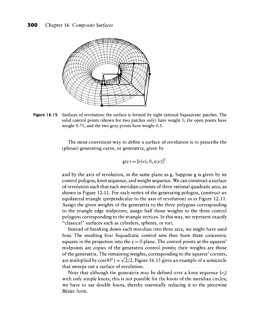
Figure 16.15 Surfaces of revolution: the surface is formed by eight rational biquadratic patches. The
solid control points (shown for two patches only) have weight 1; the open points have
weight 0.71, and the two gray points have weight 0.5.
The most convenient way to define a surface of revolution is to prescribe the
(planar) generating curve, or generatrix, given by
giv) = [riv\0,ziv)f
and by the axis of revolution, in the same plane as g. Suppose g is given by its
control polygon, knot sequence, and weight sequence. We can construct a surface
of revolution such that each meridian consists of three rational quadratic arcs, as
shown in Figure
12.11.
For each vertex of the generating polygon, construct an
equilateral triangle (perpendicular to the axis of revolution) as in Figure
12.11.
Assign the given weights of the generatrix to the three polygons corresponding
to the triangle edge midpoints; assign half those weights to the three control
polygons corresponding to the triangle vertices. In this way, we represent exactly
"classical" surfaces such as cylinders, spheres, or tori.
Instead of breaking down each meridian into three arcs, we might have used
four. The resulting four biquadratic control nets then form three concentric
squares in the projection into the z = 0 plane. The control points at the squares'
midpoints are copies of the generatrix control points; their weights are those
of the generatrix. The remaining weights, corresponding to the squares' corners,
are multiplied by cos(45°) =
%/2/2.
Fi gure 16.15 gives an example of a semicircle
that sweeps out a surface of revolution.
Note that although the generatrix may be defined over a knot sequence {Vj}
with only simple knots, this is not possible for the knots of the meridian circles;
we have to use double knots, thereby essentially reducing it to the piecewise
Bezier form.
16.8 Volume Deformations 301
1
6.8 Volume Deformations
Sometimes local control of a surface, nice as it may be, is not what is needed.
A typical design request is "stretch this surface in that direction," or "bend that
surface like so." These are global shape deformations, and the usual tweaking of
control polygon vertices is somewhat cumbersome for this task. P. Bezier devised
a method to deform a Bezier patch in a manner that would satisfy this global
deformation principle. We shall see that it is also applicable to B-spline surfaces.
For literature, see Bezier [59], [62], [63]. A more graphics-oriented version of
this principle was presented by Sederberg and Parry
[558],
see also
[268].
To illustrate the principle, let us consider the 2D case first. Let x(t) be a planar
curve (Bezier, B-spline, rational B-spline, and so forth), which is, without loss
of generality, located within the (w, v) unit square. Next, let us cover the square
with a regular grid of points hjj = [i/m^
j/^V'-,
/ = 0,.. ., m; / = 0,...,
w.
We can
now write every point (w, v) as
m n
/=0 j=0
this follows from the linear precision property of Bernstein polynomials (5.14).
If we now distort the grid of b/y into a grid
b^
y,
the point
(w,
v) will be mapped
to a point
(u^v):
m n
In other words, we are dealing with a mapping of E^ to E^.
In particular, the control vertices of the curve x(^) will be mapped to new
control vertices, which in turn determine a new curve y(^). Note that y is only
an approximation to the image of x under (16.6).^ This is highlighted by the fact
that the image of x's control polygon under (16.6) would be a collection of curve
arcs,
not another piecewise linear polygon.
We now have an indirect method for curve design: changing the b/y will
produce globally deformed curves. This technique may facilitate certain design
tasks that are otherwise tedious to perform. Figure 16.16 gives an example of
the use of this global design technique.
4 An exact procedure is described by T. DeRose
[159],