Farin G. Curves and Surfaces for CAGD. A Practical Guide

Подождите немного. Документ загружается.

272 Chapter 15 Constructing Polynomial Patches

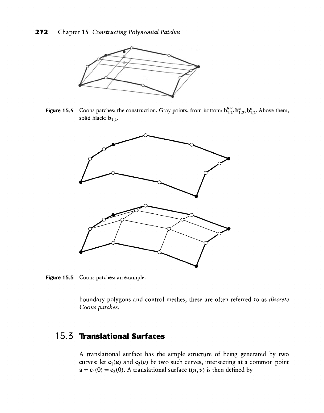
Figure 15.4 Coons patches: the construction. Gray points, from bottom:

b"'2,

Above them,

solid black:

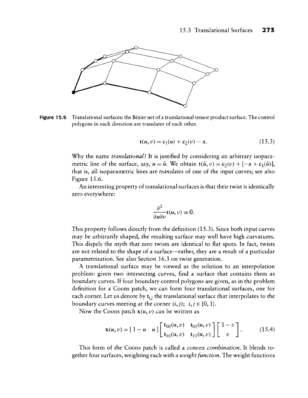
Figure 15.5 Coons patches: an example.

boundary polygons and control meshes, these are often referred to as discrete

Coons patches.

15.5 Tkranslational Surfaces

A translational surface has the simple structure of being generated by two

curves: let Ci(u) and C2(^') be tw^o such curves, intersecting at a common point

a = ci(0) = C2(0). A translational surface t(w, v) is then defined by

15.3 Translational Surfaces 273

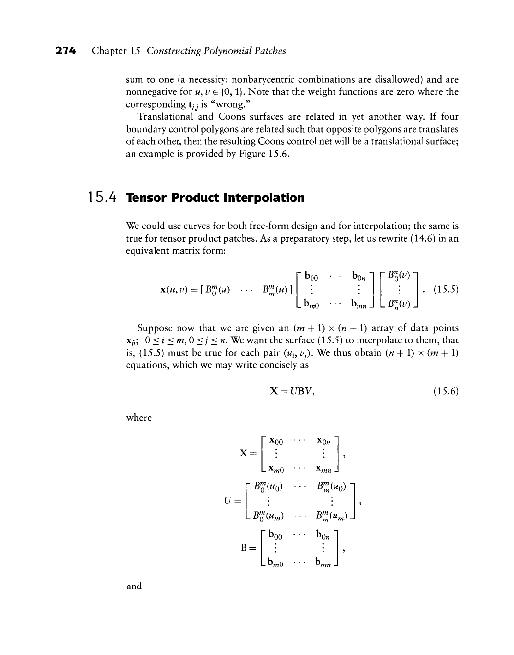
Figure 15.6 Translational surfaces: the Bezier net of

translational tensor product surface. The control

polygons in each direction are translates of each other.

t(u,

v) = Ciiu) + C2(i^) - a.

(15.3)

Why the name translational} It is justified by considering an arbitrary isopara-

metric line of the surface, say, u = u. We obtain t(w, v) = C2(i^) + [—a + Ci(ii)],

that is, all isoparametric lines are translates of one of the input curves; see also

Figure 15.6.

An interesting property of translational surfaces is that their twist is identically

zero everywhere:

dudv

t(u,

v) = 0.

This property follows directly from the definition (15.3). Since both input curves

may be arbitrarily shaped, the resulting surface may well have high curvatures.

This dispels the myth that zero twists are identical to flat spots. In fact, twists

are not related to the shape of a surface—rather, they are a result of a particular

parametrization. See also Section 16.3 on twist generation.

A translational surface may be viewed as the solution to an interpolation

problem: given two intersecting curves, find a surface that contains them as

boundary curves. If four boundary control polygons are given, as in the problem

definition for a Coons patch, we can form four translational surfaces, one for

each corner. Let us denote by tjj the translational surface that interpolates to the

boundary curves meeting at the corner (/,/); /,; €

{0,1}.

Now the Coons patch x(w, v) can be written as

x(^,

v) = [1

—

u u]

too(^, v) toi(w, v)

1-v

(15.4)

This form of the Coons patch is called a convex combination. It blends to-

gether four surfaces, weighting each with a weight function. The weight functions

274 Chapter 15 Constructing Polynomial Patches

sum to one (a necessity: nonbarycentric combinations are disallowed) and are

nonnegative for u,v e

{0,1}.

Note that the weight functions are zero where the

corresponding t^y is "wrong."

Translational and Coons surfaces are related in yet another way. If four

boundary control polygons are related such that opposite polygons are translates

of each other, then the resulting Coons control net will be a translational surface;

an example is provided by Figure 15.6.

5.4 Tensor Product Interpolation

We could use curves for both free-form design and for interpolation; the same is

true for tensor product patches. As a preparatory step, let us rewrite (14.6) in an

equivalent matrix form:

x{u,v) = [B^(u)

BZiuy

^00

LD^O

^On

Bl{v)

.B>),

(15.5)

Suppose now that we are given an (m + 1) x (w + 1) array of data points

X/y; 0 <i <m,0<j <n. We want the surface (15.5) to interpolate to them, that

is,

(15.5) must be true for each pair

(w^,

Vj).

We thus obtain (n-\-1) x (m-\- 1)

equations, which we may write concisely as

X = UBV,

(15.6)

where

XOO

^mO •

U =

boo

B =

•'mO

XOn

BZi^o)

and

v =

15.4 Tensor Product Interpolation 275

B«(t/o) ••• B"Qiv„)l

lB"Jvo)

•••

B"„{v„)}

Matrices U and V already appeared in Section 7.3; they are Vandermonde

matrices.

In an interpolation context, the x^y are known and the coefficients b/y are

unknown. They are found from (15.6) by setting

B=U-iXV-l (15.7)

The inverse matrices in (15.7) exist since the functions B^ and B^ art linearly

independent.

Equation (15.7) shows how a solution to the interpolation problem could

be found, but one should not try to invert the matrices U and V explicitly! To

solve and understand better the tensor product interpolation problem, we rewrite

(15.6) as

X = DV, (15.8)

where we have set

D=:L7B.

(15.9)

Note that D consists of (m + 1) rows and (n + 1) columns. Equation (15.8) can

be interpreted as a family of (m+1) univariate interpolation problems—one for

each row of X and D, where D contains the unknowns. Having solved all {m + 1)

problems (all having the same coefficient matrix V!), we can attack (15.9),

since we have just computed D. Equation (15.9) may be interpreted as a family

of (n + 1) univariate interpolation problems, all having the same coefficient

matrix U.

We thus see how the tensor product form allows a significant "compactifi-

cation" of the interpolation process. Without the tensor product structure, we

would have to solve a linear system of order (m

-\-

l)(n -\-1) x (m

-\-

l){n + 1).

That is an order of magnitude more complex than solving m + 1 problems with

the same (n-\-1) x (n-\-1) matrix and then solving

problems with the same

(m + 1) X (m + 1) matrix. If m = w, the naive approach would thus need O(m^)

computations, whereas the tensor product approach just needs O(m^). This will

be even more dramatic for interpolating spline surfaces.

There is a less algebraic way to describe the tensor product interpolation

process as well. Considering (15.8), we see that it may be interpreted as a family

of univariate interpolation problems with the same coefficient matrix V. That is

276 Chapter 15 Constructing Polynomial Patches

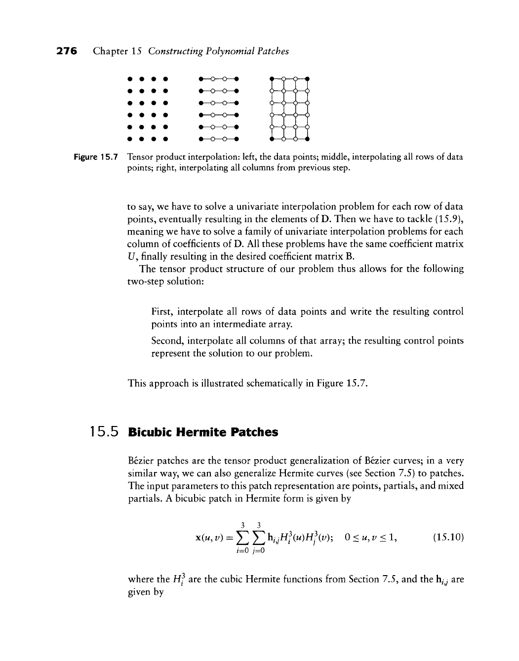
Figure 15.7 Tensor product interpolation: left, the data points; middle, interpolating all rows of data

points; right, interpolating all columns from previous step.

to say, we have to solve

univariate interpolation problem for each row of data

points, eventually resulting in the elements of D. Then we have to tackle (15.9),

meaning we have to solve

family of univariate interpolation problems for each

column of coefficients of D. All these problems have the same coefficient matrix

U, finally resulting in the desired coefficient matrix B.

The tensor product structure

our problem thus allows

for

the following

two-step solution:

First, interpolate all rows

data points and write the resulting control

points into an intermediate array.

Second, interpolate all columns of that array; the resulting control points

represent the solution to our problem.

This approach is illustrated schematically in Figure 15.7.

15.5 Bicubic Hermite Patciies

Bezier patches are the tensor product generalization

Bezier curves;

in a

very

similar way, we can also generalize Hermite curves (see Section 7.5) to patches.

The input parameters to this patch representation are points, partials, and mixed

partials. A bicubic patch in Hermite form is given by

xiu, v) =

J^Yl Kj^fMHfiv); 0<u,v<l,

(15.10)

/=0 /=0

where the

are the cubic Hermite functions from Section 7.5, and the

are

given by

15.5 Bicubic Hermite Patches 277

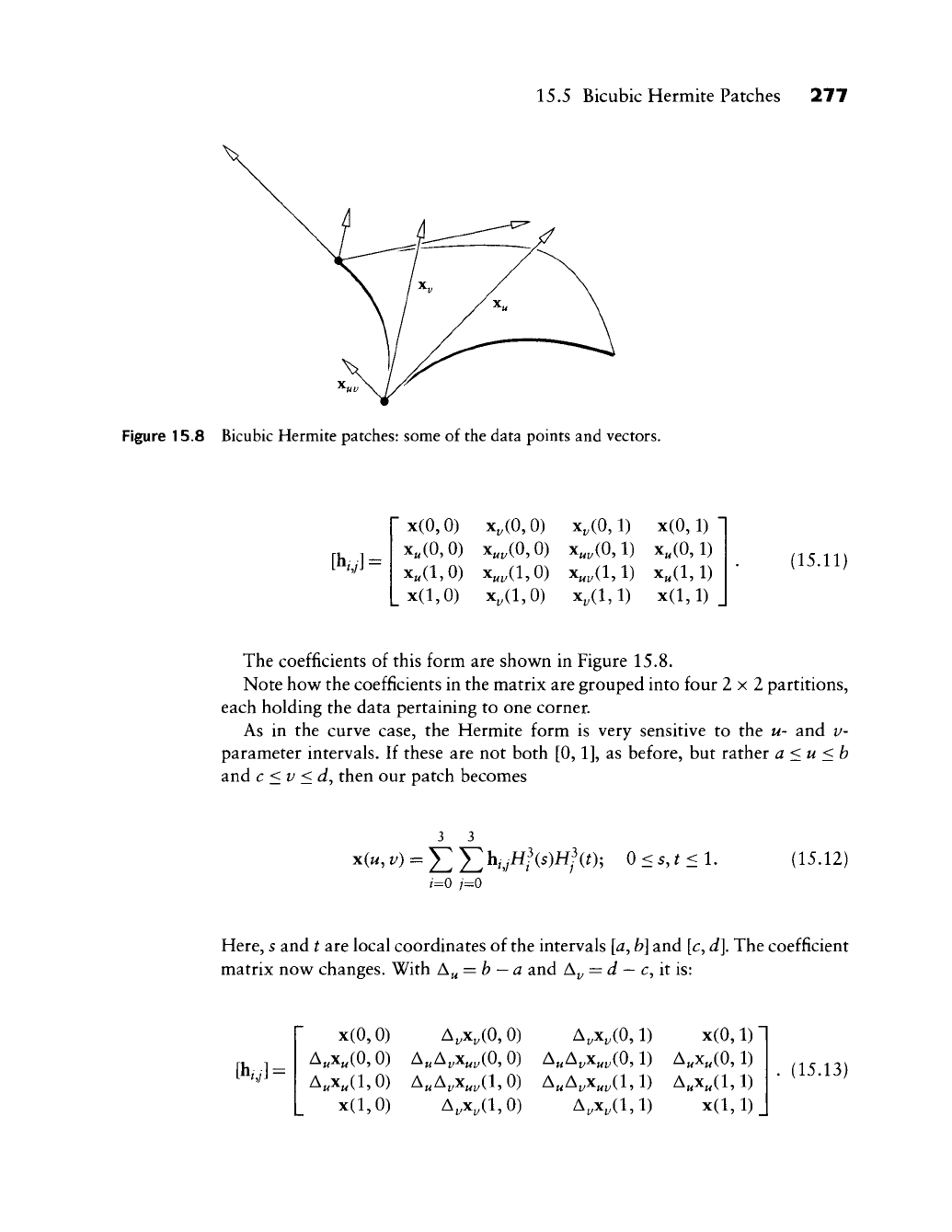
Figure 15.8 Bicubic Hermite patches: some of the data points and vectors.

[k/]=

x(0,0)

x„(0,0)

x„(l,0)

x(l,0)

x,(0,0)

x„^(0,0)

x„,(l,0)

x^(l,0)

x,(0,1)

x„,(0,1)

X„;,(l, 1)

x,(l, 1)

x(0,1)

x„(0,1)

x„(l, 1)

x(l,l)

(15.11)

The coefficients of this form are shown in Figure 15.8.

Note how the coefficients in the matrix are grouped into four 2x2 partitions,

each holding the data pertaining to one corner.

As in the curve case, the Hermite form is very sensitive to the u- and v-

parameter intervals. If these are not both

[0,1],

as before, but rather a<u<b

and c <v <d, then our patch becomes

/=0 /=0

0<s,^< 1.

(15.12)

Here, s and t art local coordinates of the intervals

[a,

and [c,

d].

The coefficient

matrix now changes. With ^^ = b

—

a and A^ = J

—

c, it is:

[k;] =

x(0,0)

A„x„(0,0)

A„x„(l,0)

x(l,0)

A,x,(0,0)

A„A^x„^(0,0)

KK^uvO-, 0)

A,x„(l,0)

A,x,(0,1)

A„A^x„j,(0,1)

x(0,1)

A„x„(0,1)

A„A„x„,/l,l) A„x„(l,l)

^u'-^v^uv\

Aj,Xj,(l, 1)

x(l,

1) J

. (15.13)

278 Chapter 15 Constructing Polynomial Patches

5.6 Least Squares

In many cases, data points do not come on a rectangular grid that ahgns with the

patch boundaries. If the data points come from a laser digitizer, for example, we

cannot expect them to have any recognizable structure whatsoever, except that

they are numbered. We are thus dealing with a set of points p^, with k ranging

from 0 to some number K—this number will typically be in the hundreds or

thousands. We also assume that each data point p^ has a corresponding pair of

parameters u^ = (w^,

Vf^).

We wish to find a Bezier patch that fits the data as good as possible. Let it be

given by a control net with coefficients b/y, with / = 0,..., m and; = 0,...,«.

Before we formulate our problem, we need to introduce a new notation.

Instead of writing a Bezier patch as a matrix product (14.23), we may intro-

duce a linearized notation. We will number all control points linearly, simply

counting them as we traverse the control net row by row. For example, we may

write a bilinear patch as

x(w, v) =

[Bl(u)Bl(v) Bliu)B\{v) B\(u)Bl(v) B\iu)B\iv)]

bo,o

bo,i

^1,0

Lbi,i_

This equation has, for the general case, (m + l)(w + 1) terms. Using this linear

ordering, our patch equation may be written as

xiu,

[

B^(u)Bl(v),..., Bl{u)Bl{v) ]

r Vo

(15.14)

Returning to our problem, we would like to achieve that each data point lies

on the approximating surface. For the kxh data point

p^,

this becomes p^ = x(u^)

^k = [B'S{Uk)Bl(vk),...,Bl{u0Bl{Vk)

•»o,o

(15.15)

Combining all K + 1 of these equations, we obtain

15.6 Least Squares

279

B^(uo)B^Jvo)

PK-i

IB^(UK)B-^(VK)

BZ(uo)B':,(vo)

BZ(UK)BI(VK)J

^0,0

^m.n

-«

We abbreviate this

(15.16)

MB.

(15.17)

These

are X + 1

equations

in (m + l)(/7 + 1)

unknowns.

For the

example

of the

bicubic case,

have

unknowns,

but

typically several hundred data points—

thus

the

linear system (15.17)

overdetermined.

will

general

not

have

exact solution,

but a

good approximation

found

forming

M^V

M^MB.

(15.18)

Our linear system

has a

square coefficient matrix

M^M^

with

(m + l)(w + 1)

rows

and

columns.

the

bilinear case,

would thus have

linear system with four equations

four unknowns,

shown

Example 15.1.

In the

bicubic case,

would have

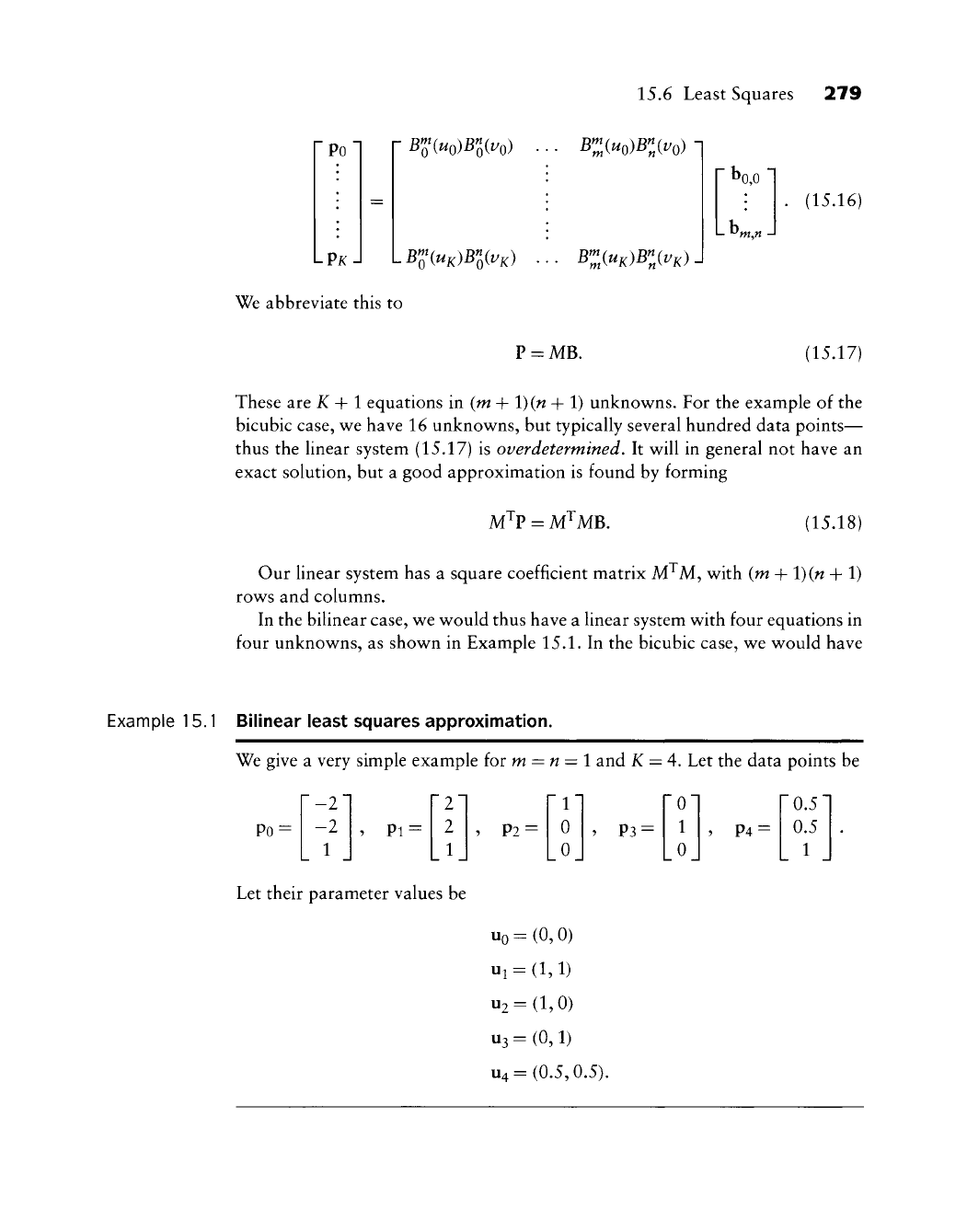
Example

15.1

Bilinear least squares approximation.

We give

very simple example

for m = n = l and K = 4. Let the

data points

~-2~

-2

Pi =

[21

P2 =

P3 =

[01

P4 =

[0.51

0.5

Let their parameter values

uo-(0,0)

= (l,l)

= (l,0)

= (0, 1)

(0.5,0.5).

280 Chapter

Constructing Polynomial Patches

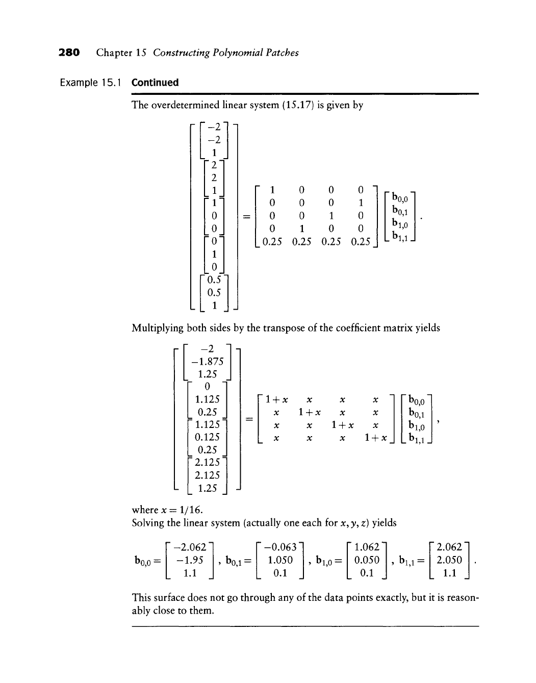
Example 15.1 Continued

The overdetermined linear system (15.17)

given

L L

•-2"

-2

[21

ril

rol

[oj

'0.5'

0.5

0.25

" bo,o

bo,i

bi,o

Lbi,iJ

Multiplying both sides

by the

transpose

the coefficient matrix yields

•

-2 •

-1.875

1.25

rol

1.125

0.25

[1.1251

0.125

0.25

[2.1251

2.125

1-25

+ x

14-x

l + x_

bo,o

bo,i

bi,o

-^1,1

where

x = 1/16.

Solving

the

linear system (actually

one

each

for x,

yields

[-2.0621

-1.95

1-1

5 Vi =

[-0.0631

1.050

0.1

\o^

[1.0621

0.050

0.1

. bi^i

[ 2.0621

2.050

1.1

This surface does

not go

through

any of

the data points exactly,

but it is

reason-

ably close

them.

15.7 Finding Parameter Values 281

to solve a linear system with 16 equations in 16 unknowns. A note of caution: if

the number of data points is very large (10^ or more), then the normal equations

become ill-conditioned and the least squares problem may not be solvable.

15.7 Finding Parameter Values

In a practical setting, we would not typically be given the parameter values

u^ = i'^h ^k)- Finding good values for the u^ is not an easy problem.

But often, the data points can be projected into a plane; let us assume they

can be projected into the x,

}/-plane

for simplicity. Each p^ is projected by simply

dropping its ;^-coordinate, leaving a pair (x^, y^). We scale the (x^, y^) so that

they fit into the unit square. Then we can simply set

uj^

xj^

and Vk^Jk-

Another solution may be obtained by using a triangulation of the data points.

This scenario is realistic for data obtained using a laser digitizer. Assuming

that the triangulation is isomorphic to the unit square, we can construct a

triangulation in the unit square with the same connectivity as the given one

in 3D.

The following method is due to Floater

[236].

First, a convex polygon is built

in the (^, v) unit square with as many vertices as the 3D mesh has boundary

vertices. This polygon is somewhat arbitray; a circle or the boundary of the unit

square is a good candidate for forming it. In this way, we assign 2D parameters

to the 3D mesh boundary points.

Next, consider any interior point u^ of the 2D mesh with

Uj.

neighbors. We call

these neighbors u^ i,. . .,

u^ „

. For a "nice" triangulation, the following condition

should be satisfied: all interior

u^.

may be expressed as^

1 "^

We now observe that there are as many equations (15.19) as there are interior

points in the mesh. Some of these equations involve boundary points, others will

not. Thus we have a linear system for the interior u^, with as many equations as

there are interior points. It is always solvable.

2 Triangulations with this property are the result of

Laplacian

smoothing of a mesh.