Farin G. Curves and Surfaces for CAGD. A Practical Guide
Подождите немного. Документ загружается.

302 Chapter 16 Composite Surfaces
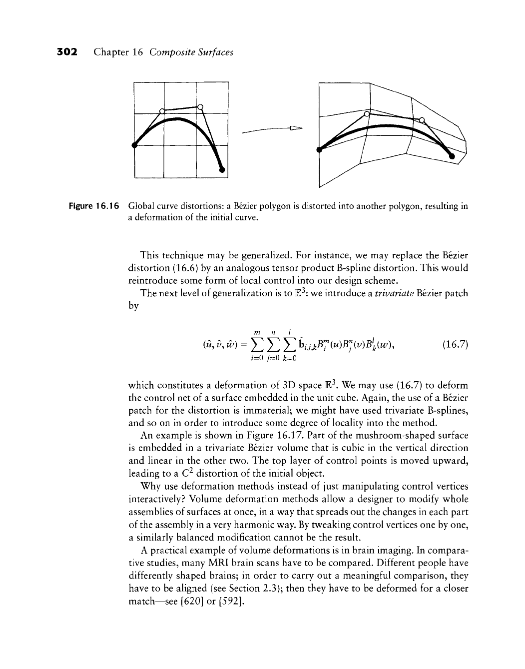
Figure 16.16 Global curve distortions: a Bezier polygon is distorted into another polygon, resulting in
a deformation of the initial curve.
This technique may be generalized. For instance, we may replace the Bezier
distortion (16.6) by an analogous tensor product B-spline distortion. This would
reintroduce some form of local control into our design scheme.
The next level of generalization is to E^: we introduce a trivariate Bezier patch
by
,=0 7=0 k=0
(16.7)
which constitutes a deformation of 3D space E-^. We may use (16.7) to deform
the control net of a surface embedded in the unit cube. Again, the use of a Bezier
patch for the distortion is immaterial; we might have used trivariate B-splines,
and so on in order to introduce some degree of locality into the method.
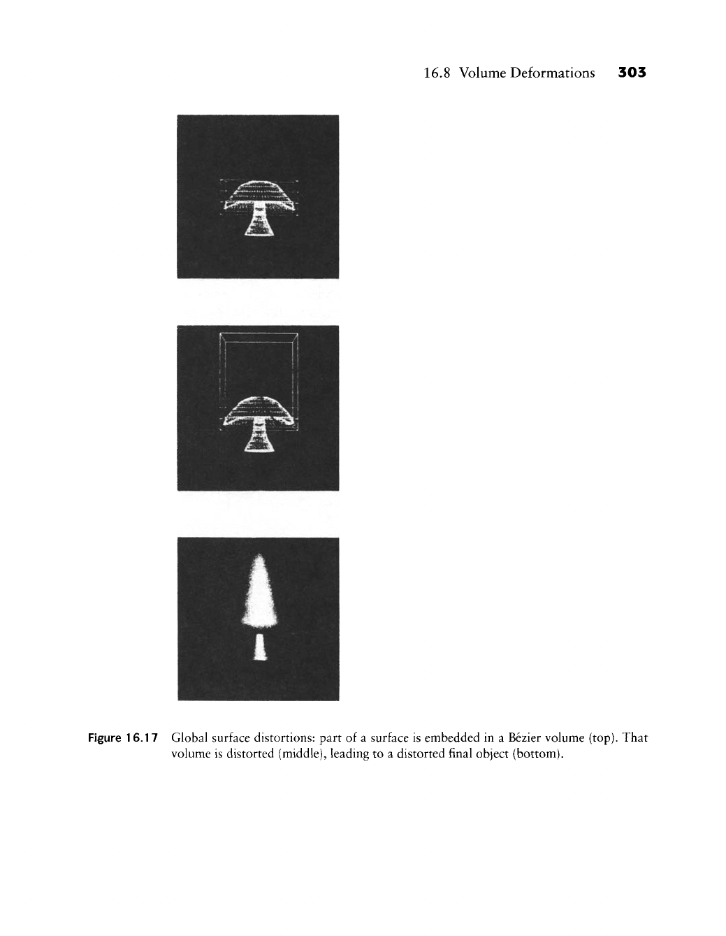
An example is shown in Figure 16.17. Part of the mushroom-shaped surface
is embedded in a trivariate Bezier volume that is cubic in the vertical direction
and linear in the other two. The top layer of control points is moved upward,
leading to a C^ distortion of the initial object.
Why use deformation methods instead of just manipulating control vertices
interactively? Volume deformation methods allow a designer to modify whole
assemblies of surfaces at once, in a way that spreads out the changes in each part
of the assembly in a very harmonic way. By tweaking control vertices one by one,
a similarly balanced modification cannot be the result.
A practical example of volume deformations is in brain imaging. In compara-
tive studies, many MRI brain scans have to be compared. Different people have
differently shaped brains; in order to carry out a meaningful comparison, they
have to be aligned (see Section 2.3); then they have to be deformed for a closer
match—see [620] or
[592].
16.8 Volume Deformations 303
Figure 16.17 Global surface distortions: part of a surface is embedded in a Bezier volume (top). That
volume is distorted (middle), leading to a distorted final object (bottom).
304 Chapter 16 Composite Surfaces
16.9 CONS and Trimmed Surfaces
If we create any parametric curve
{u{t)^
v{t)) in the domain of a surface x(w, i/),
it will be mapped to a curve x(u(t), v(t)) on the surface, or CONS. If the domain
curve is itself
a
Bezier curve of degree p, then the CONS will be of degree (m + n)p,
assuming m and n are the parametric degrees of x(w, v). Such curves were first
considered by Bezier, see [57], [60], where they were called transposants.
In most practical applications, the curve in the domain is expressed as a piece-
wise linear curve, and the resulting CONS is approximated as being piecewise
linear. If the piecewise linear CONS is dense enough, this should not cause prob-
lems.
CONS can arise in many applications: if we intersect two surfaces, the
resulting intersection curve is a CONS on either of the two surfaces. Or we could
project a space curve onto a surface, again resulting in a CONS.
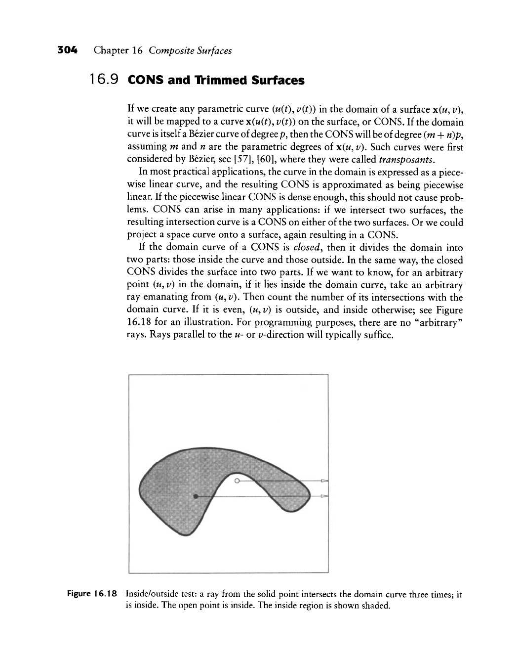
If the domain curve of a CONS is
closed,
then it divides the domain into
two parts: those inside the curve and those outside. In the same way, the closed
CONS divides the surface into two parts. If we want to know, for an arbitrary
point (u, v) in the domain, if it lies inside the domain curve, take an arbitrary
ray emanating from (w, v). Then count the number of its intersections with the
domain curve. If it is even, («, v) is outside, and inside otherwise; see Figure
16.18 for an illustration. For programming purposes, there are no "arbitrary"
rays.
Rays parallel to the u- or i/-direction will typically suffice.
Figure 16.18 Inside/outside test: a ray from the solid point intersects the domain curve three times; it
is inside. The open point is inside. The inside region is shown shaded.
16.9 CONS and Trimmed Surfaces 305
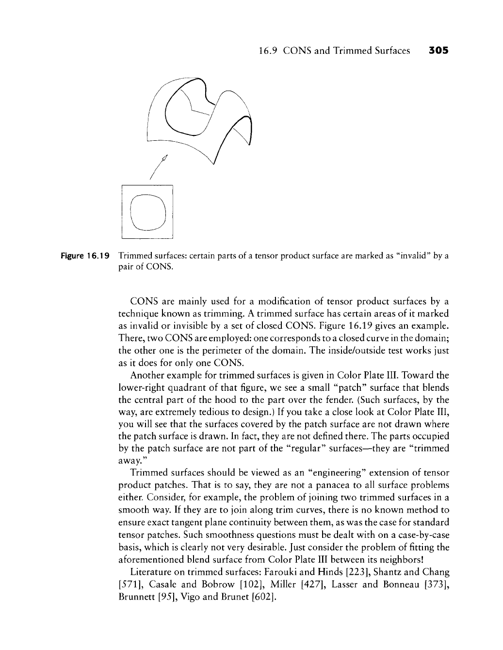
Figure 16.19 Trimmed surfaces: certain parts of a tensor product surface are marked as "invalid" by a
pair of CONS.
CONS are mainly used for a modification of tensor product surfaces by a
technique known as trimming. A trimmed surface has certain areas of it marked
as invalid or invisible by a set of closed CONS. Figure 16.19 gives an example.
There, two CONS are employed: one corresponds to a closed curve in the domain;
the other one is the perimeter of the domain. The inside/outside test works just
as it does for only one CONS.
Another example for trimmed surfaces is given in Color Plate III. Toward the
lower-right quadrant of that figure, we see a small "patch" surface that blends
the central part of the hood to the part over the fender. (Such surfaces, by the
way, are extremely tedious to design.) If you take a close look at Color Plate III,
you will see that the surfaces covered by the patch surface are not drawn where
the patch surface is drawn. In fact, they are not defined there. The parts occupied
by the patch surface are not part of the "regular" surfaces—they are "trimmed
away."
Trimmed surfaces should be viewed as an "engineering" extension of tensor
product patches. That is to say, they are not a panacea to all surface problems
either. Consider, for example, the problem of joining two trimmed surfaces in a
smooth way. If they are to join along trim curves, there is no known method to
ensure exact tangent plane continuity between them, as was the case for standard
tensor patches. Such smoothness questions must be dealt with on a case-by-case
basis,
which is clearly not very desirable. Just consider the problem of fitting the
aforementioned blend surface from Color Plate III between its neighbors!
Literature on trimmed surfaces: Farouki and Hinds
[223],
Shantz and Chang
[571],
Casale and Bobrow
[102],
Miller
[427],
Lasser and Bonneau
[373],
Brunnett [95], Vigo and Brunet
[602].
306 Chapter 16 Composite Surfaces
16.10 Implementation
The routines in this section are written for rational surfaces. By setting all weights
equal to one, the standard piecewise polynomial case is recovered.
The routine that converts a rational bicubic B-spline control net into the
piecewise bicubic Bezier form:
void ratbspl_to_bez_surf(bspl_x,bspl_y,bspl_w,lu,lv,knot_u,
knot_v,bez_x,bez_y,bez_w,dux_x,aux_y,aux_w)
/*
Converts B-spline control
net
into piecewise
Bezier control
net
(bicubic).
Input: bspl_x,bspl_y: B-spline control
net
(one coordinate only)
bspl_w: B-spline weights
lu,lv: no.
of
intervals
in u-
and
v-directi on
knot_u, knot_v: knot vectors
in u-
and
v-directi on
Output: bez_x,bez_y: piecewise bicubic Bezier net.
bez_w: Bezier weights.
Work space:aux_x,aux_y,aux_w: needed
to
store intermediate results.
Remark:
The
piecewise Bezier
net
only stores each control point once,
i.e., neighboring patches share
the
same boundary.
Knots
are
simple (but,
in
the
language
of
Chapter 10,
the
boundary knots have multiplicity
three).
V
Once the piecewise rational Bezier representation of a bicubic spline surface
is achieved, the following routine plots the whole surface:
void piot_ratbez_surfaces(bez_x,bez_y,bez_w,1u,1v,u_points,v_points,
seale_x,scale_y,val ue)
/* Plots piecewise cubic surface,
i.e.,
generates postscript output
Input: bez_x, bez_y: control nets
lu,lv:
no. of
segments
in u- and v-
direction
u_points,v_points:
per
patch: v_points many
isoparametric curves with
u_points
points
on
each
value:
minmax
box of all
control nets,
seale_x,seale_y: scale factors
for
postscript
V
Tensor product spline interpolation (bicubic) is carried out by the following
routine. It uses Bessel end conditions.

16.10 Implementation 307
void spline_surf_int(data_x,data_y,bspl__x,bspl_y,lu,lv,knot_u,
knot_v,aux_x,aux_y)
/*
Interpolates
to an
array
of
size [0,lu+2]x[0,lv+2]
Input: data_x, data_y: data array (one coordinate only)
lu,lv: no.
of
intervals
in u- and
v-directi on
knot_u, knot_v: knot vectors
in u- and
v-directi on
Output: bspl_x,bspl_y: B-spline control
net.
Work space: aux_x, aux_y.
Remark:
On
input,
it is
assumed that data_x
and
data_y have rows
1
and
lu+1
and
columns
1 and
lv+1 empty, i.e., they
are
not filled with data points. Example
for
lu=4,
lv=7:
xOxxxxxxOx
0000000000
xOxxxxxxOx x=data coordinate,
xOxxxxxxOx 0=unused input array
xOxxxxxxOx element.
0000000000
The O's
will
be
filled with
xOxxxxxxOx 'tangent Bezier points'.
This approach makes
it
easy
to
feed
in
clamped
end
conditions
if
so
desired:
put in
values
in the O's and
delete
the
calls
to bessel_ends below.
V
Next is the header of a program that plots the control net of a Bezier surface
or of a composite surface.
void psplot_net(lu,lv,bx,by,step_u,step_v,seale_x,seale_y,value)
/* plots control net into postscript-file.
Input: lu,lv: dimensions of net
bXjby: net vertices
step_u,step_v: subnet sizes (e.g. both=3 for pw bicubic net)
scale_x,scale_y:scale factors for ps
value:
window size in world coords
Output: written into postscript file
V
308 Chapter 16 Composite Surfaces
16.11 Problems
1 Generalize the B-spHne knot insertion algorithm to the tensor product case.
* 2 Show that if two polynomial surfaces are across a common boundary,
then they are also twist continuous across that boundary.
* 3 Suppose we want to find a parametrization [uj] for a tensor product in-
terpolant. We may parametrize all rows of data points and then form the
averages of the parametrizations thus obtained. Or we could average all
rows of data points, for example, by setting p^ = J^j n^ij ^^^ ^^ could
then parametrize the
p^.
Do we get the same result? Discuss both methods.
P1 Embed your Bezier surface from Problem
P3
of Chapter 14 in a tricubic grid,
similar to Figure 16.17. Then "stretch" your surface, leaving the front part
unchanged.
P2 Model a Klein bottle as a closed bicubic B-spline surface. Literature:
[323],
[170].
If you have the graphics capabilities, display your result as a translu-
cent surface.
P3 Generate an array of points on a sphere. For latitudes, take 0/ = 0,10,20,
..., 90 degrees. For longitudes, take
i/zj
= 45,50,55,..., 75 degrees. Pass
several tensor product interpolants through the data and compare their
deviations from the true sphere. For the bicubic C^ spline interpolant, also
compare uniform and chord length parametrizations.
Bezier Triangles
When de Casteljau invented Bezier curves in 1959, he realized the need for the
extension of the curve ideas to surfaces. Interestingly enough, the first surface
type that he considered was what we now call Bezier triangles. This historical
"first" of triangular patches is reflected by the mathematical statement that they
are a more "natural" generalization of Bezier curves than are tensor product
patches. We should note that although de Casteljau's work was never published,
Bezier's was; therefore, the corresponding field now bears Bezier's name. For
the placement of triangular Bernstein-Bezier surfaces in the field of CAGD, see
Barnhill [24].
Though de Casteljau's work (established in two internal Citroen technical
reports [145] and [146]) remained unknown until its discovery by W. Boehm
around 1975, other researchers realized the need for triangular patches. M. Sabin
[516] worked on triangular patches in terms of Bernstein polynomials, unaware
of de Casteljau's work. Among the people concerned with the development of
triangular patches we name L. Frederickson
[249],
P. Sablonniere
[522],
and D.
Stancu
[580].
All of their Bezier-type approaches relied on the fact that piecewise
surfaces were defined over regular triangulations; arbitrary triangulations were
considered by Farin
[189].
Two surveys on the field of triangular Bezier patches
are Farin [197] and de Boor
[139].
17.1 The de Casteljau Algorithm
The de Casteljau algorithm for triangular patches is a direct generalization of
the corresponding algorithm for curves. The curve algorithm uses repeated linear
interpolation, and that process is also the key ingredient in the triangle case. The
309
310 Chapter 17 Bezier Triangles
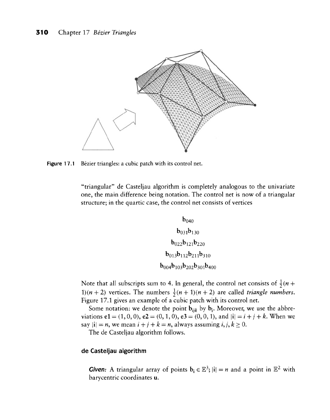
Figure 17.1 Bezier triangles: a cubic patch with its control net.
"triangular" de Casteljau algorithm is completely analogous to the univariate
one,
the main difference being notation. The control net is now of a triangular
structure; in the quartic case, the control net consists of vertices
bo40
^031^130
^022^121^220
boi3bll2b21lb3io
^0041^103^202^301^400
Note that all subscripts sum to 4. In general, the control net consists of j(n +
l)(n + 2) vertices. The numbers j(n + l)(w + 2) are called triangle numbers.
Figure 17.1 gives an example of a cubic patch with its control net.
Some notation: we denote the point b/y^ by bj. Moreover, we use the abbre-
viations el =
(1,
0,0), e2 = (0,1, 0), e3 = (0,0,1), and |i| =i + j + k. When we
say |i| = w, we mean / + / + fe = w, always assuming /, /, k>0.
The de Casteljau algorithm follows.
de Casteljau algorithm
Given: A triangular array of points h[ € E^; |
barycentric coordinates u.
: n and a point in E^ with
17.1 The de Casteljau Algorithm 311
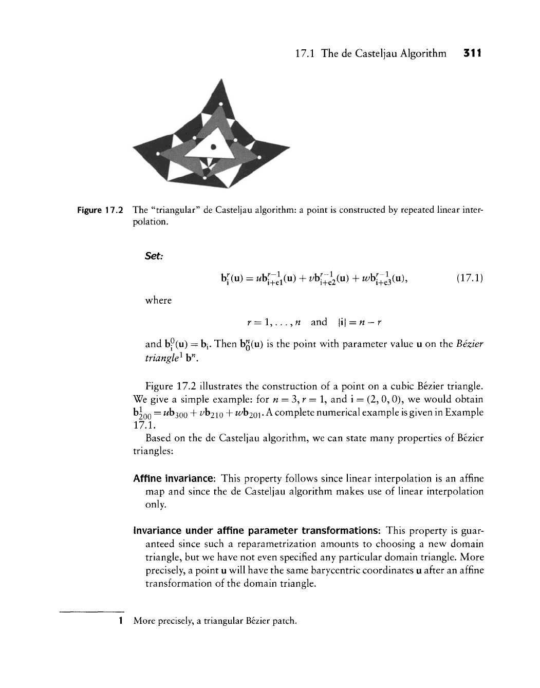
Figure 17.2 The "triangular" de Casteljau algorithm: a point is constructed by repeated linear inter-
polation.
Set;
where
br(u) = «b[;^V") + ^K;e2(") + ^K;e3(")' d^'D
r =
l,...,w
and \i\=n
—
r
and bP(u) =
h[.
Then bgCu) is the point with parameter value u on the Bezier
triangle^ b".
Figure 17.2 illustrates the construction of a point on a cubic Bezier triangle.
We give a simple example: ior n = 3^r = 1, and i = (2, 0, 0), we would obtain
b^QQ
=
uh^QQ
H-
i^b2io + ^b2oi- A complete numerical example is given in Example
17.1.
Based on the de Casteljau algorithm, we can state many properties of Bezier
triangles:
Affine invariance: This property follows since linear interpolation is an affine
map and since the de Casteljau algorithm makes use of linear interpolation
only.
Invariance under affine parameter transformations: This property is guar-
anteed since such a reparametrization amounts to choosing a new domain
triangle, but we have not even specified any particular domain triangle. More
precisely, a point u will have the same barycentric coordinates u after an affine
transformation of the domain triangle.
1 More precisely, a triangular Bezier patch.