Douce A.P. Thermodynamics of the Earth and Planets

Подождите немного. Документ загружается.

288 Phase equilibrium and phase diagrams

Note that (6.1) and (6.3) are two different functions that yield the value of the same extensive

property, Z. Taking the derivative of (6.3):



∂Z

∂T



P ,n

dT +



∂Z

∂P



T ,n

dP +





∂Z

∂n



P ,T ,n

j≡i

. (6.4)

Substituting the definition of partial molar property, equation (5.28), in (6.4), equating with

(6.2) and simplifying we arrive at the following, known as the Gibbs–Duhem equation:



∂Z

∂T



P ,n

dT +



∂Z

∂P



T ,n

dP −



=0. (6.5)

This equation is valid for any thermodynamic extensive variable, but its most common

application is to Gibbs free energy, in which case, by using (4.132) and (4.133), it becomes:

dT −V

dP +



dµ

=0. (6.6)

In this form equation (6.6) is also known as Gibbs’equation 97. Dividing by the total number

of mols, n

we can also write the Gibbs–Duhem equation as follows:

dT −V

dP +



dµ

=0. (6.7)

The Gibbs–Duhem equation specifies the number of intensive variables that can vary inde-

pendently in a homogeneous phase in thermodynamic equilibrium. For example, suppose

that we can describe the composition of a phase in terms of the amounts of s different chem-

ical species. There are then s +2 intensive variables in (6.6): pressure, temperature and the

chemical potential of each of the s species. The equation has s +1 degrees of freedom,

which is the number of intensive variables that must be specified in order to solve it.

You may have noticed that, whereas in Chapter 5 we distinguished between system com-

ponents and phase components, in the previous paragraph we ignored that distinction and

referred simply to the chemical species that make up the phase. The reason for this is that

the Gibbs–Duhem equation makes no distinction between phase components and system

components. We imposed no restrictions on the type of components when writing equation

(6.1), except that whichever components we choose must allow us to fully describe the com-

position of the phase. Thus, the Gibbs–Duhem equation is equally true whether we choose

to describe the composition of the phase in terms of system components, phase components

or any combination of the two. We will exploit this flexibility on many occasions.

6.1.2 Gibbs’ phase rule

Consider now a system made up of F different phases, and let us describe the composition

of each of the phases in terms of the same set of system components. Recall from Section

5.1.1 that this is a set of chemical species whose compositions are linearly independent and

such that they span the composition space of the full system (and hence of each of the phases

that make up the system). In the language of linear algebra the system components conform

a coordinate basis or minimal spanning set for the composition space of the system. The

coordinate basis, i.e. the specific set of system components that we choose, is not unique

289 6.1 The foundations of phase equilibrium

but, importantly, whatever basis we choose it always contains the same number of system

components, which we shall call c (in linear algebra, c is the dimension of the composition

space). We can construct a system of F Gibbs–Duhem equations, as follows:

dT −V

dP +



i=1

dµ

.............................................. (6.8)

dT −V

dP +



i=1

dµ

=0.

For a system at equilibrium, and given that we have chosen to write all of the Gibbs–Duhem

equations in terms of the same set of system components, it must be µ

=···=µ

, for

every one of the c components, 1 ≤ i ≤ c. At equilibrium there must also be identity

among the differentials of the chemical potentials, i.e. dµ

=···=dµ

. There are then

F equations in c + 2 independent variables: dT, dP and cdµs. Two fundamental results

follow immediately from the elementary algebraic properties of systems of linear equations.

(i) The maximum possible number of phases at equilibrium in a system composed of c

linearly independent chemical species (= system components)isc + 2. If the number

of phases, F, were greater than this then there would be more Gibbs–Duhem equations

than independent variables and the system of equations would be inconsistent.

(ii) The number of degrees of freedom of the system, f , is given by:

f =c +2 −F. (6.9)

The number of degrees of freedom, f ≥ 0, also called the variance of the system, is

the number of intensive variables that must be specified, or constrained independently,

in order to be able to solve the system of equations (6.8) and hence have a complete

description of the thermodynamic state of the system.

These two statements constitute Gibbs’ phase rule. It is a simple algebraic result with

profound implications for understanding the physicochemical constitution of planetary

bodies.

The phase rule is commonly derived along the lines that I followed here, but I find it

interesting that a subtle yet obvious question is seldom addressed explicitly: where does

the 2 in equation (6.9) come from? Perhaps the clearest justification for the 2 can be found

intheveryfirsttwosectionsofGuggenheim’sThermodynamics(1967),whichIrephrase

as follows:

In order to specify the thermodynamic state of a system we need a variable that keeps

track of changes in thermal energy – temperature or its conjugate, entropy – and another

variable that keeps track of changes in mechanical energy – pressure or its conjugate,

volume. These are the two variables that show up in equation (6.9) in addition to the

chemical potentials of each of the linearly independent chemical species.

If additional products of conjugate variables need to be considered (see Section 4.8.4), such

as would be the case if the gravitational potential cannot be ignored (Chapter 13), then the

constant term in equation (6.9) becomes greater than 2.

290 Phase equilibrium and phase diagrams

6.1.3 Choosing and switching components

The solution of a system of equations such as (6.8) yields a “complete thermodynamic

description” of the system of interest. By this we mean that we can calculate its pressure,

its temperature and the chemical potential of each of the chemical species that compose the

system. Equivalently, since there is a functional relationship between chemical potential

and composition (e.g., equation (5.2.12)), the “complete thermodynamic description” could

be T, P and the composition of each phase. This is the most useful description in planetary

sciences, and the chief goal of many thermodynamic calculations. There are alternative

ways of arriving at this description. One possibility is to integrate each of the Gibbs–Duhem

equations in (6.8) and then solve for the combination of intensive variables that satisfies the

system of integrated equations. This is seldom easy, especially for systems of more than two

components. Fortunately, it is also seldom necessary, as several shortcuts are possible. In

fact, we have already used some of these shortcuts in the numerical examples in Chapter 5.

In the derivation of the phase rule we specified that the Gibbs–Duhem equations for all

phases in the system be written in terms of system components. Because system compo-

nents constitute a minimal spanning set for the composition of the system, this requirement

assures that the number of unknown variables in the system of equations (6.8) is the mini-

mum possible. The number of equations relating these variables in (6.8) is also the minimum

possible, as there is one and only one Gibbs–Duhem equation per phase. These two state-

ments signify that the mathematical description of the thermodynamic state of the system is

complete and cannot be simplified any further. In particular, regardless of the way in which

we choose to solve for the thermodynamic state of the system, the number of degrees of

freedom of our system of equations must be the one given by the phase rule. This is perhaps

the most important consequence of Gibbs’ phase rule, and the first key to finding algebraic

shortcuts for the thermodynamic description of a system.

The second key is more a question of intuition, experience and the specific goal that one

has, rather than a rigorous mathematical rule, although such rule exists, as we shall see in a

moment. We begin by choosing the set of chemical species that we are actually interested

in. This is determined by the nature of the system that we are investigating, and by what we

know about the possible compositional range of each of the phases that make up the system.

We must choose at least as many chemical species as the number of system components,

and we must choose a set of chemical species that allows us to write the composition of all

of the phases in the system. Beyond these restrictions, however, there can be any number of

species, and their nature (system components, phase components or a combination of both)

is not important. Let us say that we choose a total of s chemical species, with s ≥ c (c is

the number of system components). The F Gibbs–Duhem equations must be re-written in

terms of these s components (some of the mol numbers or mol fractions may be zero, but

this is not a problem).

Clearly, ifs > c then the compositions of all s species cannot be linearly independent. More

precisely, there must exist s–clinearly independent equations relating the compositions of

the s species. Each of these equations corresponds to a balanced chemical reaction among

some or all of the s chemical species. But if we can write a balanced chemical reaction among

chemical species then we can also write an equation among their chemical potentials that

describes a condition of heterogeneous chemical equilibrium. Each of these equations is a

version of (5.22):



=0 (6.10)

291 6.1 The foundations of phase equilibrium

and each one can be differentiated to obtain an equation of the form:



dµ

=0. (6.11)

There are s–cequations like (6.11), which, together with the F Gibbs–Duhem equations,

gives a total of F +s–cequations. These equations contain s+2 unknown variables:

pressure, temperature and the chemical potential of each of the s chemical species. The

number of degrees of freedom of the augmented system of equations is still c+2 – F,

as required by the phase rule. This system of equations is an alternative description of the

thermodynamic state of the system that is equivalent to a set of Gibbs–Duhem equations

such as (6.8).

The underlying algebraic rule is simple: we must add one equation for each chemical

species that we wish to consider beyond the number of system components. Generally,

each of these additional equations is an equation of heterogeneous equilibrium of the form

(6.10). And the shortcut that we seek is to solve only these equations, and stay away from

the Gibbs–Duhem equations if at all possible. Equations of the form (6.10) are a lot easier

to solve because they are already given in integral form, and all that is required is a function

that gives chemical potential in terms of P, T and phase composition. This is exactly what

we have been doing throughout Chapter 5.

By now you may be thoroughly confused. The best way of clearing the air is with

an example. I encourage you to go over the following example carefully, and return to

the preceding discussion often as you do so. The example also demonstrates additional

thermodynamic possibilities that we will exploit further in subsequent sections.

Worked Example 6.1 The spinel–garnet transition in planetary mantles revisited

The model for the spinel–garnet transition that we discussed in Chapter 5 consists of the

four phases: spinel, orthopyroxene, olivine and garnet. The Mg end-member system is

spanned by three system components, which we can choose as SiO

,Al

and MgO (but

see Exercise 6.1). Thus, F = 4, c = 3 and, from (6.9), f = 1. This is the same number of

degrees of freedom that we found when we solved the equations that describe the phase

boundaries in Worked Examples 5.1 and 5.6. Where did those equations come from, and

how can we be sure that they are a complete thermodynamic description of the system?

Let us start by writing out the Gibbs–Duhem equations in terms of our chosen system

components. The explicit form of (6.8) for this system is:

dT −V

dP +n

SiO

dµ

SiO

dµ

MgO

dµ

MgO

opx

dT −V

opx

dP +n

opx

SiO

dµ

SiO

opx

dµ

opx

MgO

dµ

MgO

dT −V

dP +n

SiO

dµ

SiO

dµ

MgO

dµ

MgO

grt

dT −V

grt

dP +n

grt

SiO

dµ

SiO

grt

dµ

grt

MgO

dµ

MgO

=0. (6.12)

I have omitted the phase identification subscripts in the chemical potential terms because

at equilibrium the chemical potential of each component is the same in all phases. Some

of the mol numbers, such as n

SiO

and n

, may be zero, but there is no harm in keep-

ing the corresponding terms in (6.12). This is a (minimal) system of four equations with five

unknowns: dP, dT, dµ

SiO

,dµ

and dµ

MgO

. We could solve it by integrating the

292 Phase equilibrium and phase diagrams

Gibbs–Duhem equations and specifying the value of any one of the intensive variables. As

an aside, a system of equations such as (6.12), in which all equations have a zero constant

term, is called a homogeneous system and its only solutions are zeroes. Integrating the

equations converts (6.12) into a heterogeneous system with non-zero solutions, thanks to

non-zero integration constants. This is an important concept from linear algebra, but need

not concern us too much at this point for, if all we are interested in is the location of the

phase boundary, there is a much easier solution that does not require any integration.

We begin by re-writing the Gibbs–Duhem equations in terms of an appropriately chosen

set of phase components. Suppose first that we did not know thatAl can enter orthopyroxene.

The compositions of the four phases can in that case be written out in terms of the four

phase components: MgAl

,Mg

SiO

and Mg

. This is one more

than the number of system components, so in order to preserve the number of degrees of

freedom we must add an equation. Let us re-write the Gibbs–Duhem equations in terms of

our new set of components:

dT −V

dP +n

MgAl

dµ

MgAl

opx

dT −V

opx

dP +n

opx

dµ

opx

dT −V

dP +n

SiO

dµ

SiO

grt

dT −V

grt

dP +n

grt

dµ

grt

=0. (6.13)

In (6.13) it is convenient to include the phase identification subscripts in the chemical

potentials because the additional equation that we seek is a heterogeneous equilibrium

equation among these species, obtained by differentiation of equation (5.23):

MgAl

+2µ

opx

=µ

grt

+µ

SiO

, (6.14)

which results in:

dµ

MgAl

+2dµ

opx

−dµ

grt

−dµ

SiO

=0. (6.15)

Equations (6.13) and (6.15) constitute a system of five equations in six unknowns: dP, dT

and the four dµs. It therefore preserves the one degree of freedom required by the phase rule,

as shown by the system (6.12). We do not need to solve the full system of equations, however,

because we can write each of the chemical potentials in (6.14) as a function of temperature

and pressure. For phases in their standard state (e.g. pure phase at the temperature and

pressure of interest) the required function µ

= µ

(P , T ) is equation (5.1.1). Substituting

a function of this kind for each of the four phases in (6.14) reduces this equation to two

unknowns: P and T. The resulting equation is (5.16), which we solved in Worked Example

5.1 by specifying temperature.

Of course, we know from Worked Example (5.6) that, given that Al dissolves in

orthopyroxene, this solution is not correct. In order to obtain a better solution we need to

consider an additional chemical species, the Mg–Tschermak’s component in orthopyroxene:

MgAlAlSiO

. The Gibbs–Duhem equations are now as follows:

dT −V

dP +n

MgAl

dµ

MgAl

opx

dT −V

opx

dP +n

opx

dµ

opx

MgAlAlSiO

dµ

MgAlAlSiO

opx

293 6.1 The foundations of phase equilibrium

dT −V

dP +n

SiO

dµ

SiO

grt

dT −V

grt

dP +n

grt

dµ

grt

=0. (6.16)

But, in order to preserve the number of degrees of freedom we need an additional equation,

which is the heterogeneous equilibrium condition for reaction (5.102):

MgAl

spinel

+µ

opx

=µ

MgAlAlSiO

opx

+µ

SiO

olivine

. (6.17)

or, equivalently:

dµ

MgAl

spinel

+dµ

opx

−dµ

MgAlAlSiO

opx

+dµ

SiO

olivine

=0. (6.18)

Equations (6.16), (6.15) and (6.18) constitute a system of six equations in seven unknowns:

dP, dT and five dµs. Hence, one degree of freedom (and J. Willard Gibbs stays happy). But

if we now focus on the integral forms of (6.15) and (6.18), which are equations (6.14) and

(6.17), respectively, we see that these are two equations in three unknowns, as we can write

the chemical potentials of Mg

and MgAl

SiO

as a function of P, T and mol fraction

of Mg (or Al) in orthopyroxene, and all the other chemical potentials as functions of P and

T only. With the appropriate substitutions, and assuming ideal mixing in orthopyroxene, the

resulting equations are (5.101) and (5.103), which we solved in Worked Example 5.6. Note

that if we choose to treat orthopyroxene as a non-ideal solution there is still one degree

of freedom, as the excess chemical potentials of Mg

and MgAl

SiO

are functions

of P, T and orthopyroxene composition only (e.g. equations (5.153)or(5.154)) so that no

additional variables are introduced (this is true in general, not just for this specific example).

There is no need to stop here, however. For example, we may be interested in the chem-

ical potentials of the species SiO

,Al

and MgO. Even though the amounts of these

components cannot vary independently in any of the four phases that we are considering,

equations (6.12) assure us that the chemical potentials of these species are well defined,

and can be calculated. It is important to understand that this is always true, even if none

of these chemical species exist as “free” or “stoichiometric” components in the system of

interest. We will have many uses for this fact. For now, we motivate the following calcula-

tion by noting that the chemical potentials of the oxide species may be important in order

to understand how mantle phases interact with supercritical hydrous fluids (Chapter 9), or

in order to understand their melting relationships (Chapter 10).

Since we have already determined that equations (6.14) and (6.17) by themselves consti-

tute a valid thermodynamic description of our system we can start from these two equations

only and ignore the Gibbs–Duhem equations. The problem of determining the chemical

potentials of the three oxides is simply one of adding three new variables: µ

SiO

, µ

and µ

MgO

and three new equations of heterogeneous equilibrium, so as to preserve the

number of degrees of freedom. There are several possible sets of equations, but as long as

we choose three equations that are linearly independent which particular three we choose

is immaterial (Exercise 6.3). Here I choose the following three:

SiO

+SiO

 Mg

(6.19)

2MgAl

+SiO

 Mg

SiO

+2Al

(6.20)

MgAl

 MgO +Al

. (6.21)

294 Phase equilibrium and phase diagrams

We can write the chemical potential of each of the three oxides as the sum of its standard

state chemical potential, chosen, for example, as pure crystalline solid at the temperature and

pressure of interest, plus an activity term (equation (5.45)). The conditions of heterogeneous

chemical equilibrium for the three reactions are then as follows:



0,(6.19)

P,T

+RT ln



Mg,M1



opx

−RT ln a

SiO

=0 (6.22)



0,(6.20)

P,T

+2RT ln a

−RT ln a

SiO

=0 (6.23)



0,(6.21)

P,T

+RT ln a

MgO

=0. (6.24)

In these equations the standard state chemical potentials of the oxides are included in the



G terms, as usual. I have assumed ideal mixing in orthopyroxene and used (5.99) for

the activity of Mg

. We now have five equations: (6.14), (6.17) and (6.22) through

(6.24), with six independent variables: P, T, X

Mg,M

SiO

and a

MgO

. The system of

equations preserves the single degree of freedom and can be solved if we specify the value

of one of the intensive variables. It is straightforward to add the three new equations to

the Maple worksheet that we developed in Software Box 5.4 to solve for the spinel–garnet

phase boundary. We can then specify temperature (for example) and solve simultaneously

for the other five variables. You should verify (Exercises 6.2 and 6.3) that the resulting

values of pressure and Al content in orthopyroxene are the same ones that we obtained in

Chapter 5 (Fig. 5.10).

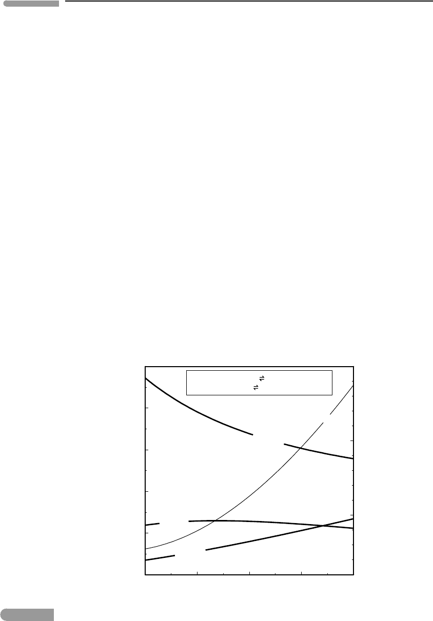
The activities of the three oxides calculated in this way are plotted in Fig. 6.1 as a function

of temperature. In the ternary SiO

–Al

–MgO system, the four-phase assemblage spinel–

orthopyroxene–olivine–garnet fixes, or buffers, the chemical potentials (or activities) of the

three oxide components along the curves shown in Fig. 6.1. This means that, as long

800 1000 1200 1400 1600

0.2

0.4

0.6

0.8

T(°C)

activity

a(Al

)

a(MgO)

a(SiO

)

spinel+ 2 enstatite forsterite+ pyrope

spinel+ enstatite

Mg-tsch+ forsterite

P (kbar)

Fig. 6.1 Activities of Al

, SiO

and MgO buffered by the orthopyroxene–spinel–forsterite–pyrope univariant assemblage.

Pressure at the univariant equilibrium from Fig. 5.10.

295 6.2 Analysis of phase equilibrium

as the four phases are present, the chemical potential of each oxide takes one and only one

value at any given temperature. Note that neither pressure nor (X

Mg,M1

)

opx

are constant

along these curves. Rather, their values are the equilibrium values for each temperature, as

shown in Fig. 5.10.

The three oxides behave differently with temperature. In particular, the activity of Al

increases with decreasing temperature, and reaches a value of 1 at T ∼750

◦

C and P ∼17.5

kbar. Since the standard state that we chose is pure crystalline Al

at the temperature

and pressure of interest, this means that at those P–T conditions the four-phase system

becomes saturated in an additional phase, namely, corundum. According to the phase rule

the number of degrees of freedom now becomes zero, as the number of system components

has not changed, but there is now an additional phase. A system of equations with no

degrees of freedom has a single solution and does not allow us to fix the value of any of the

variables independently. Thus, in the ternary SiO

–Al

–MgO system there is a single

P–T combination at which the five phases spinel–orthopyroxene–olivine–garnet–corundum

coexist at equilibrium. We discuss these concepts further beginning in Section 6.2.

You may be wondering, why do we need to go to all the trouble discussed in excruciating

detail in this example? In practice we seldom do, as we tacitly skip over the Gibbs–Duhem

equations (unless there are reasons to use them, more on this later). However, before immers-

ing oneself in any thermodynamic calculation it is always necessary to do a “phase rule

check” of number of phases, components and degrees of freedom (and of course the Gibbs–

Duhem equations are implicit in this). If the number of degrees of freedom of whatever

system of equations we set up does not agree with the number predicted by the phase rule

then our proposed thermodynamic description cannot be correct.

As another example, consider the gas speciation calculation from Worked Examples 5.4

and 5.5. Our model system consists of two phases (graphite and gas) and is described by two

system components (we can choose, for example, C and O

). Thus, Gibbs’phase rule assures

us that the system has two degrees of freedom. When we solved the system of equations

consisting of (5.87), (5.88) and the composition of the gas phase (X

=1)

I stated that this is a system of three equations in three unknowns (the three mol fractions),

that can therefore be solved exactly. This does not mean, however, that the thermodynamic

system has no degrees of freedom, as in order to solve this system of equations we had to

specify two intensive variables: temperature and pressure (which we fixed at 1 bar). The

thermodynamic system has two degrees of freedom, as required by the phase rule. The

species distribution can only be calculated if we specify both P and T.

6.2 Analysis of phase equilibrium among phases of

ﬁxed composition

The phase rule is the foundation for the study of phase equilibrium and phase diagrams.

For the sake of clarity it is convenient to break up the discussion of phase diagrams into

different parts, focusing first on equilibria among phases of fixed composition and then on

equilibria among phases of variable composition. Nature, of course, does not fall neatly into

one or the other of these categories, so that we generally have to keep both sets of concepts

in mind.

296 Phase equilibrium and phase diagrams

6.2.1 Some fundamental concepts and terminology

A phase assemblage with a single degree of freedom (such as the four-phase assemblage

spinel–orthopyroxene–olivine–garnet in the ternary system SiO

–Al

–MgO) is called a

univariant assemblage. Recall that this means that, if the four phases exist at equilibrium,

then only one intensive variable can be independently specified. The geometric representa-

tion of a univariant assemblage is a segment of a curve, that we also call a phase boundary

(e.g. Figs. 5.2 and 5.5). It should be immediately apparent that an assemblage with no degrees

of freedom, called an invariant assemblage, is expressed geometrically by a point, and an

assemblage with two degrees of freedom, termed divariant, is represented geometrically

by a sector of a two-dimensional surface. We could keep going, and note that a trivariant

assemblage corresponds to a portion of a three-dimensional volume, a quadrivariant assem-

blage to a portion of a four-dimensional hypervolume, and so on. Algebraic descriptions

of assemblages with any number of degrees of freedom are not a problem, but phase dia-

grams limit us to representing information in two dimensions. This means that geometric

representations of phase equilibria commonly do not extend beyond divariant assemblages.

This would appear to be a serious limitation on the usefulness of phase diagrams but, as

we shall soon see, in most cases it is not, as it allows us to focus on those variables that

are particularly relevant to the problem at hand. Moreover, low-variance assemblages (say,

those with f ≤ 2) are particularly useful, as they often make it possible to place fairly tight

brackets on the values of intensive variables.

An equilibrium invariant assemblage (f = 0) in a system of c components consists of

c +2 phases (equation (6.9)). This assemblage is represented by a point on a plane, in which

the coordinates are any two intensive variables. The emphasis is crucial: the variables that

we use to track phase equilibrium can be any combination of intensive variables, and the

principles that rule the construction of phase diagrams are the same regardless of which

combination of intensive variables we use. The variables can be P and T, or two chemical

potentials, or a chemical potential and T or P, or some other combination. In order to

emphasize the fact that the rules that govern phase diagrams are completely general I will

use the names Y and Z for the intensive variables, unless the specific example calls for a

particular set of intensive variables. Going back now to our system of c components we

can see that there are c + 2 different univariant assemblages that converge at the invariant

point, each of them consisting of c + 1 phases. We obtain these univariant assemblages by

eliminating each of the c + 2 phases that exist at the invariant point, one at a time. Each of

these univariant assemblages is represented by a different curve on the Y−Z plane, and all

of the curves must have a common intersection at the invariant point.

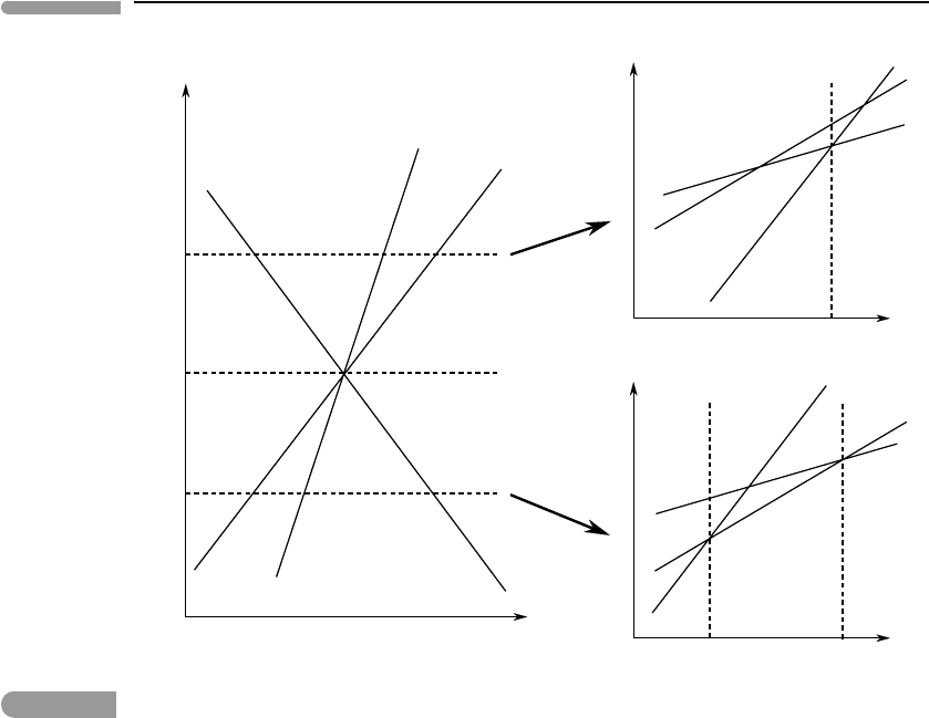
Consider now a system of one component, in which there are three phases: A, B and C,

that exist at equilibrium at an invariant point. There are three univariant curves that intersect

at the invariant point, each of them representing univariant equilibrium of one of the three

possible two-phase assemblages. This situation is sketched in the left hand side of Fig. 6.2.

The labels next to the univariant curves indicate which phases are stable on each side of each

phase boundary, and the two phases are of course stable along the corresponding curve. This

particular arrangement of phases is not random. It is an arrangement that is thermodynam-

ically possible. In order to see what this means, and to derive some fundamental properties

of phase diagrams, we begin by noting that Gibbs free energy is a monotonic function of

all intensive variables or, more precisely, that the first and second derivatives of Gibbs free

energy relative to any intensive variable never change sign. We have seen that this is the

case for temperature and pressure (equations (4.132), (4.133), (4.135) and (4.136)), and it is

297 6.2 Analysis of phase equilibrium

123

Fig. 6.2

Univariant equilibria in a one-component system shown as a function of the intensive variables Z and Y (left). Each

point on the univariant curves corresponds to an intersection between two G = G(Y) curves at constant Z (right

diagrams). For example, intersection 2 between the Gibbs free energy curves for phases A and B corresponds to the

point on the A–B univariant curve at Z =Z

and Y =Y

AB.

trivial to show (e.g. from equation (6.1)) that it is also true for the derivatives of G relative

to chemical potential. This property of the Gibbs free energy function means that, if Y and

Z are any two intensive variables and Z is kept constant, then the curves G = G(Y ) for

different univariant assemblages intersect only once. This is shown on the right-hand side

of Fig. 6.2, for two different values of Z, greater than and less than the value of Z at the

invariant point, Z

Clearly, the three G(Y ) curves have a common intersection point at the (Y, Z ) coordinates

of the invariant point (not shown in the figure). It is also evident that, because G is monotonic

relative to all intensive variables, the order in which the curves intersect relative to the value

of Y must change as the value of Z becomes greater or less than that at the invariant point.

For example, for Z

> Z

the order of intersection may be as shown in the top right of Fig.

6.2. If this is the case, then there must exist a finite interval in the neighborhood of the

invariant point, Z

< Z

, in which the curves intersect as shown in the bottom right of

Fig. 6.2. It follows that some arrangements of univariant and divariant assemblages around

the invariant point are possible, whereas others are not thermodynamically permissible.

The monotonicity of the Gibbs free energy function assures us of this. Note that it would

be equally valid to have the sequence of intersections be 1–2–3 at Z

and 4–5–6 at Z

However, given the properties of the Gibbs free energy function, other arrangements are

not possible (see also Exercise 6.4).