Davidson K.R., Donsig A.P. Real Analysis with Real Applications

CHAPTER 13

Fourier Series and Physics

Fourier series were ﬁrst developed to solve partial differential equations that arise

in physical problems, such as heat ﬂow and vibration. We will look at the physics

problem of heat ﬂow to see how Fourier series arise and why they are useful. Then

we will proceed with the solution, which leads to a lot of very interesting mathe-

matics. Then we will see that the problem of a vibrating string leads to a different

PDE that requires similar techniques to solve.

While this problem sounds very applied, the inﬁnite series that arise as solu-

tions forced mathematicians to delve deeply into the foundations of analysis. When

d’Alembert proposed his solution for the motion of a vibrating string in 1754, there

were no clear, precise deﬁnitions of limit, function, or even of the real numbers—

all things taken for granted in most calculus courses today. D’Alembert’s solution

(which we shall see at the end of this chapter) has a closed form, and thus did not

really challenge deep principles. However, the solution to the heat problem that

Fourier proposed in 1807 required notions of convergence that mathematicians of

that time did not have. Fourier won a major prize in 1812 for this work, but the

judges, Laplace, Lagrange, and Legendre, criticized Fourier for lack of rigour.

Work in the nineteenth century by many now famous mathematicians eventually

resolved these questions by developing the modern deﬁnitions of limit, continuity,

and uniform convergence. These tools were developed not because of some fetish

for ﬁnding complicated things, but because they were essential to understanding

Fourier series.

13.1. The Steady-State Heat Equation

The purpose of this section is to derive from physical principles the partial

differential equation satisﬁed by heat ﬂow on a surface.

Consider the problem of determining the temperature on a thin metal disk given

that the temperature on the boundary circle is ﬁxed. We assume that there is no

heat loss in the third dimension. Perhaps this disk is placed between two insulating

pads. We also assume that the system is at equilibrium. As a consequence, the

423

424 Fourier Series and Physics

temperature at each point remains constant over time. This is known as the steady-

state heat problem.

It is convenient to work in polar coordinates in order to exploit the symmetry.

The disk will be given as the set

D = {(x, y) : x

+ y

≤ 1} = {(r, θ) : 0 ≤ r ≤ 1, −π ≤ θ ≤ π},

where (0, θ) represents the origin for all values of θ; and (r, −π) = (r, π) for

all r ≥ 0. More generally, we allow (r, θ) for any real value of θ and make the

identiﬁcation (r, θ + 2π) = (r, θ).

Let us denote the temperature distribution over the disk by a function u(r, θ),

and let the given function on the boundary circle be f(θ).

As usual in physical problems such as this, we need to know a mathematical

form of the appropriate physical law in order to determine a differential equation

that governs the behaviour of the system. In this case, the law is that the heat ﬂow

across a boundary is proportional to the temperature difference between the two

sides of the curve. Of course, our temperature distribution function will be contin-

uous. So we must deal with the inﬁnitesimal version of temperature change, which

is the derivative of the temperature in the direction perpendicular to the boundary,

known as the normal derivative.

With this assumption, we can write down a mathematical version of the fact

that given any region R in the disk with piecewise smooth boundary C, the total

amount of heat crossing the boundary C must be 0. This yields the heat conservation

equation

0 =

∂u

∂n

ds.

Here ∂u/∂n denotes the normal derivative in the outward direction perpendicular

to the tangent, and ds indicates integration over arc length along the curve.

Those students comfortable with multivariable calculus will recognize a ver-

sion of the Divergence Theorem:

∂u

∂n

ds =

∆u dA,

where ∆u = u

is the Laplacian and dA represents integration with respect

to area. Whenever a continuous function integrates to 0 over every nice region

(say squares or disks), then the function must be 0 everywhere, which leads to

the equation ∆u = 0. This is the desired differential equation, except that it is

necessary to express the Laplacian in polar coordinates. A (routine but nontrivial)

exercise using the multivariate chain rule shows that

∆u = u

θθ

For the convenience of students unfamiliar with ideas in the previous para-

graph, we show how to derive this equation directly. This has the advantage that

we can work in polar coordinates and avoid the need for a messy change of vari-

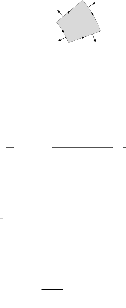
ables. The idea is to take R to be the region graphed in Figure 13.1, namely

R = {(r, θ) : r

≤ r ≤ r

, θ

≤ θ ≤ θ

13.1 The Steady-State Heat Equation 425

Then we will divide the integral by (θ

− θ

)(r

− r

) and take the limit as θ

decreases to θ

and r

decreases to r

, which we evaluate using the Fundamental

Theorem of Calculus. This will yield the same result.

FIGURE 13.1. The region R with boundary and outward normal vectors.

The boundary C of R consists of two radial line segments

= {(r, θ

) : r

≤ r ≤ r

} and L

= {(r, θ

) : r

≤ r ≤ r

}

and two arcs

= {(r

, θ) : θ

≤ θ ≤ θ

} and A

= {(r

, θ) : θ

≤ θ ≤ θ

Taking orientation into account, C = L

+ A

− L

− A

. Along L

, the outward

normal at (r, θ

) is in the θ direction, and arc length along the circle with angle h

is rh, thus

∂u

∂n

(r, θ

) = lim

h→0

u(r, θ

+ h) − u(r, θ

)

(r, θ

Along the arc A

, the outward normal is the radial direction, and thus the normal

derivative is u

, θ). The arc length ds along the radii L

and L

is just dr, while

arc length along an arc of radius r is r dθ. Thus by adding over the four pieces of

the boundary, we obtain the conservation law

0 =

(r, θ

) − u

(r, θ

)

dr +

, θ)r

dθ −

, θ)r

dθ

(r, θ

) − u

(r, θ

)

dr +

, θ) − r

, θ)

dθ.

Divide by θ

− θ

and take the limit as θ

decreases to θ

. The ﬁrst term

is integrated with respect to r, which is independent of θ, and thus the limit is

evaluated using the Leibniz Rule (8.3.4). For the second term, the limit follows

from the Fundamental Theorem of Calculus.

0 =

lim

→θ

(r, θ

) − u

(r, θ

)

− θ

+ lim

→θ

− θ

, θ) − r

, θ)

dθ

θθ

(r, θ

) dr + r

, θ

) − r

, θ

)

426 Fourier Series and Physics

Now divide by r

− r

and take the limit as r

decreases to r

. We obtain

0 = lim

→r

− r

θθ

(r, θ

) dr +

, θ

) − r

, θ

)

− r

θθ

, θ

) +

∂

∂r

(ru

)(r

, θ

)

θθ

, θ

) + u

, θ

) + r

, θ

)

= r

∆u(r

, θ

Thus our differential equation with boundary conditions becomes

∆u := u

θθ

= 0 for 0 ≤ r < 1, −π ≤ θ ≤ π

u(1, θ) = f (θ) for − π ≤ θ ≤ π.

Exercises for Section 13.1

A. Do the change of variables calculation converting u

+ u

to polar coordinates.

B. Let u(r, θ) = log r. Compute ∆u and u(1, θ). Explain why u is not a solution of the

heat equation for the boundary function f(θ) = 0.

C. Suppose that u is a solution of the steady-state heat equation for the annulus A =

{(r, θ) : r

≤ r ≤ r

(a) If u depends only on r, and not on θ, what ODE does u satisfy? Solve the heat

equation for the boundary conditions u(r

, θ) = a

and u(r

, θ) = a

(b) Show that if u depends only on θ, then it is constant.

D. Show that u(r, θ) = (3−4r

)+(8r

−8r

) sin

θ+8r

sin

θ satisﬁes ∆u(r, θ) = 0

and u(1, θ) = 8sin

θ.

E. Let S = {(x, y) : 0 ≤ x ≤ 1, y ∈ R} and consider the steady-state heat problem on

this strip.

(a) Show that e

nπy

sinnπx is a solution for the problem of zero boundary values.

(b) Do you believe that this is a reasonable solution to the physical problem? Discuss.

F. Suppose that an inﬁnite rod has a temperature distribution u(x, t) at the point x ∈ R

at time t > 0. The heat equation is u

= u

(a) Prove that u(x, t) =

√

4πt

−x

/4t

is a solution.

(b) Evaluate the total heat at time t:

∞

−∞

u(x, t) dx.

HINT: Let I =

∞

−∞

−x

dx. Express I

as a double integral over the plane, and

convert to polar coordinates. Or use Example 8.3.5.

t→0

u(x, t). Can you give a physical explanation of what this limit repre-

sents?

13.2 Formal Solution 427

13.2. Formal Solution

The steady-state heat equation is a difﬁcult problem to solve. We approach it

ﬁrst by making the completely unjustiﬁed assumption that there will be solutions

of a special form. Then we combine the solutions we ﬁnd to obtain a quite general

solution in which all considerations of convergence are ignored. After that, we

will work backward and show rigorously that these solutions in fact make good

sense and are completely general. So we justify our ﬁrst steps as experiments that

lead us to a likely candidate for the solution but do not in themselves constitute a

proper derivation of the solution. In subsequent sections, we will use our analysis

techniques to justify why it works.

Our method, called separation of variables, is to look for solutions of the form

u(r, θ) = R(r)Θ(θ), where R is a function only of r and Θ is a function only of θ.

The reason for doing this is that it enables us to split the partial differential equation

into two ordinary differential equations of a single variable each. Indeed, the DE

∆u = 0 becomes

(r)Θ(θ) +

R(r)Θ

(θ) = 0.

Manipulate this by taking all dependence on r to one side of the equation and all

dependence on θ to the other to obtain

(r) + rR

(r)

R(r)

−Θ

(θ)

Θ(θ)

The left-hand side does not depend on θ and the right-hand side does not depend

on r. As they are equal, they are both independent of all variables and hence are

equal to a constant c.

(r) + rR

(r)

R(r)

= c =

−Θ

(θ)

Θ(θ)

These equations can now be rewritten as

(θ) + cΘ(θ) = 0

and

(r) + rR

(r) − cR(r) = 0.

The ﬁrst equation is a well-known linear DE with constant coefﬁcients. We

know from Section 12.6 that this DE has a two-parameter space of solutions corre-

sponding to the possible initial values. We can solve the equation (D

+ cI)y = 0

making use of the quadratic equation x

+ c = 0, which has roots ±

√

−c if c < 0,

a double root at 0 for c = 0 and two imaginary roots ±

√

ci when c > 0. Hence by

Exercise 12.6.B, we obtain the solutions

Θ(θ) = A cos(

√

c θ) + B sin(

√

c θ) for c > 0

Θ(θ) = A + Bθ for c = 0

Θ(θ) = Ae

√

−c θ

+ Be

−

√

−c θ

for c < 0.

428 Fourier Series and Physics

However, not all of these solutions ﬁt our problem. Our solutions must be 2π-

periodic because (r, −π) and (r, π) represent the same point; and more generally

(r, θ) and (r, θ + 2π) represent the same point. Hence

Θ(−π) = Θ(π) and Θ

(−π) = Θ

(π).

This eliminates the case c < 0 and limits the c = 0 case to the constant functions.

For c > 0, this forces

√

c to be an integer. Hence we obtain

Θ(θ) = A cos nθ + B sinnθ for c = n

≥ 1

Θ(θ) = A for c = 0.

Now for each c = n

, n ≥ 0, we must solve the equation

(r) + rR

(r) − n

R(r) = 0.

This is not as easy to solve, but a trick, the substitution r = e

, leads to the answer.

Differentiation yields

= R

and

= (R

r + R

)r = r

+ rR

Hence our DE becomes

= n

R. This is a linear DE with constant coefﬁcients,

which has the solutions

R = ae

+ be

−nt

= ar

+ br

−n

for n ≥ 1

R = a + bt = a + b logr for n = 0.

Again physical considerations demand that R be continuous at r = 0. This elim-

inates the solutions r

−n

and logr. That leaves the solutions R(r) = ar

for each

n ≥ 0.

Combining these two solutions for each c = n

provides the solutions

u(r, θ) = A

cosnθ + B

sinnθ for n ≥ 0.

Of course, the case n = 0 is special and yields u(r, θ) = A

. Since the sum of

solutions for a homogeneous DE such as ours will also be a solution, we obtain a

formal solution (ignoring convergence issues)

u(r, θ) = A

∞

n=1

cosnθ + B

sinnθ.

Continuing to ignore the question of the convergence, we let r = 1 and use our

boundary condition to obtain

f(θ) = A

∞

n=1

cosnθ + B

sinnθ.

Such a series is called a Fourier series, which we have discussed in Section 7.4.

13.3 Orthogonality Relations 429

Exercises for Section 13.2

A. (a) Verify that ∆u = 0 = ∆v implies that ∆(au + bv) = 0 for all scalars a, b ∈ R.

(b) Solve the DE y

= −y

. Show that the sum of any two solutions can never be a

solution.

B. Adapt the method of this section (i.e., separation of variables) to ﬁnd the possible

solutions of ∆u(r, θ) = 0 on the region U = {(r, θ) : r > 1} that are continuous on

and are continuous at inﬁnity in the sense that lim

r→∞

u(r, θ) = L exists, independent

of θ.

C. Let HS = {(x, y) : 0 ≤ x ≤ 1, y ≥ 0}, and consider the steady-state heat problem

on HS with boundary conditions u(0, y) = u(1, y) = 0 and u(x, 0) = x − x

(a) Use separation of variables to obtain a family of basic solutions.

(b) Show that the conditions on the two inﬁnite bounding lines restricts the possible

solutions. If in addition, you stipulate that the solution must be bounded, express

the resulting solution as a formal series.

D. Consider a circular drum membrane of radius 1. At time t, the point (r, θ) on the

surface has a vertical deviation of u(r, θ, t). The wave equation for the motion is

= c

∆u, where c is a constant. In this exercise, we will only consider solutions

that have radial symmetry (no dependence on θ).

(a) What boundary condition should apply to u(1, θ, t)?

(b) Look for solutions to the PDE of the form u(r, θ, t) = R(r)T (t). Use separation of

variables to obtain ODEs for R and T . An unknown constant must be introduced.

(a reasonable physical hypothesis)?

(d) The DE for R is called Bessel’s DE. What degeneracy of the DE requires us to add

another condition that R remain bounded at r = 0?

13.3. Orthogonality Relations

The next step in our heuristic development is to determine the coefﬁcients A

and B

in the Fourier series given in the last section. To do this, we use the natural

inner product on C[−π, π] given by

hf, gi =

2π

−π

f(θ)g(θ) dθ.

In Section 7.4, we showed that the functions {1,

√

2cosnθ,

√

2sinnθ : n ≥ 1}

form an orthonormal set in C[−π, π] with this inner product.

Moreover, we used the orthogonality relations to show that for a trigonometric

polynomial p(θ) = A

k=1

coskθ + B

sinkθ, we can recover all of the

coefﬁcients from the inner products A

= hp, 1i, A

= hp, 2 cos kθi and B

hp, 2sinkθi for k ≥ 1. This was the motivation for deﬁning Fourier series of

430 Fourier Series and Physics

f ∈ C[−π, π] to be

f ∼ A

∞

k=1

coskθ + B

sinkθ,

where A

= hf, 1i =

2π

−π

f(t) dt, A

= hf, 2 cos kθi =

−π

f(t) coskt dt

and B

= hf, 2 sin kθi =

−π

f(t) sinkt dt for k ≥ 1.

We have said nothing yet about the convergence of this series. There are serious

difﬁculties that need to be addressed. We also note that this deﬁnition makes sense

when f is not continuous provided that f is Riemann integrable. Since f must be

bounded,

kfk

2π

−π

|f(θ)|dθ < ∞.

Such functions are called absolutely integrable functions. In particular, Fourier

series of piecewise continuous functions are deﬁned. We will need the following

easy estimate.

13.3.1. LEMMA. If f is absolutely integrable on [−π, π], then

| ≤ kf k

, |A

| ≤ 2kf k

and |B

| ≤ 2kf k

for n ≥ 1.

Since kfk

≤ kfk

∞

, it follows that if f ∈ C[−π, π], then its Fourier coefﬁcients

are bounded.

PROOF. This is routine. For example,

| ≤

−π

|f(θ) sinnθ|dθ ≤

−π

|f(θ)|dθ = 2kf k

Moreover, it is evident that if f is bounded,

kfk

2π

−π

|f(θ)|dθ ≤

2π

−π

kfk

∞

dθ = kfk

∞

So continuous functions are absolutely integrable, and thus the Fourier coefﬁcients

are bounded by 2kfk

∞

. ¥

13.3.2. EXAMPLE. Consider the Fourier series of the function f(θ) = |θ| for

−π ≤ θ ≤ π. First note that f is even, so that f(θ) sinnθ is an odd function for all

n ≥ 1. Hence B

= 0 for all n ≥ 1 (Exercise 13.3.G). For A

we compute

2π

−π

|t|dt =

t dt =

13.3 Orthogonality Relations 431

and, using integration by parts,

−π

|t|cosnt dt =

t cosnt dt

sinnt

−

sinnt

dt = 0 +

2cosnt

πn

(−1)

− 1







0 if n is even

−

πn

if n is odd.

Thus the Fourier series is

|θ| ∼

−

∞

k=0

cos(2k + 1)θ

(2k + 1)

Exercises for Section 13.3

A. Find the Fourier series of the following functions:

(a) f(θ) = cos

(θ)

(b) f(θ) = |sinθ|

B. Find the Fourier expansion for the function u(r, θ) of Exercise 13.1.D with boundary

function f(θ) = sin

θ.

C. Verify the remaining parts of Lemma 7.4.5.

D. (a) Suppose that f(θ) is a 2π-periodic function with known Fourier series. Let α be a

real number, and let g(θ) = f(θ − α) for θ ∈ R. Find the Fourier series of g.

(b) Combine part (a) with Exercise A(b) to ﬁnd the Fourier series of |cosθ|.

E. (a) Let f(θ) be a 2π-periodic function with a given Fourier series. Let g(θ) = f (−θ)

for θ ∈ R. Find the Fourier series of g.

(b) Suppose that h is a 2π-periodic function such that h(π − θ) = h(θ). What does

this imply about its Fourier series?

F. (a) Compute the Fourier series of f(θ) =

(

1 − |θ| for − 1 ≤ θ ≤ 1

0 otherwise

(b) Compute the Fourier series of g(θ) =











1 for − 1 ≤ θ ≤ 0

−1 for 0 < θ ≤ 1

0 otherwise

G. Show that if f ∈ C[−π, π] is an odd function, then the Fourier series of f involves

only functions of the form sinkθ. Similarly, if f ∈ C[−π, π] is an even function, then

the Fourier series of f involves only the constant term and the cosine functions.

H. For f ∈ C[−π, π], deﬁne f

(θ) =

f(θ) + f (−θ)

and f

(θ) =

f(θ) − f (−θ)

Compute the Fourier series of f

and f

in terms of the series for f.

432 Fourier Series and Physics

I. Show that f

(θ) = 1 and f

(θ) =

√

2cos nθ on 0 ≤ θ ≤ π for n ≥ 1 is an orthonor-

mal set in C[0, π] for the inner product hf, gi =

f(θ)g(θ) dθ.

J. (a) Find an inner product on C[0, 1] so that {

√

2sin nπx : n ≥ 1} is an orthonormal

set, and verify that this set is orthonormal for your choice of inner product.

(b) In Exercise 13.2.C, ﬁnd the coefﬁcients necessary to satisfy the boundary condition

on the unit interval.

13.4. Convergence in the Open Disk

It is now time to return to the original problem and systematically analyze our

proposed solutions. The behaviour of the function u on the open disk

D = {(r, θ) : 0 ≤ r < 1, −π ≤ θ ≤ π}

is much easier than the analysis of the boundary behaviour. We deal with that ﬁrst,

and we will ﬁnd that it leads to a method for understanding the Fourier series of f.

Often results about the behaviour of u on D will follow from a stronger result on

each smaller closed disk

= {(r, θ) : 0 ≤ r ≤ R, −π ≤ θ ≤ π} for R < 1.

13.4.1. PROPOSITION. Let f be an absolutely integrable function on [−π, π]

with Fourier series f ∼ A

∞

n=1

cosnθ + B

sinnθ. Then the series

∞

n=1

cosnθ + B

sinnθ

converges uniformly on

for any R < 1 and thus converges everywhere on the

open disk D to a continuous function u(r, θ).

PROOF. This follows from the Weierstrass M-test (8.4.7). Indeed,

cosnθ + B

sinnθ

= max

(r,θ)∈

cosnθ + B

sinnθ

≤ (|A

| + |B

|)R

≤ 4kf k

Since

∞

n=0

4kfk

1 − R

< ∞,

the M-test guarantees that the series converges uniformly on D

. The uniform

limit of continuous functions is continuous by Theorem 8.2.1. Therefore, u(r, θ) is

continuous on D

. Since this is true for each R < 1, u is continuous on the whole

open disk D. ¥

Davidson K.R., Donsig A.P. Real Analysis with Real Applications

Подождите немного. Документ загружается.