Davidson K.R., Donsig A.P. Real Analysis with Real Applications
Подождите немного. Документ загружается.


11.1 Fixed Points and the Contraction Principle 333
x
∗
so that for every point x in (a, b) except for x
∗
itself, the orbit O(x) always
leaves the interval U.
Notice that for an attractive fixed point x
∗
, the interval U around x
∗
may be
quite small. Also, for a repelling fixed point x
∗
, the orbit O(x) may return to the
interval U after it leaves. However, it must then leave the interval again eventually.
We shall see that if T is differentiable, the difference between attractive and
repelling fixed points comes down to the size of the derivative at x
∗
. A fixed point
x
∗
is attracting if |T
0
(x
∗
)| < 1 and repelling if |T
0
(x
∗
)| > 1. The case |T
0
(x
∗
)| = 1
is ambiguous and might be one, the other, or neither.
In our example,
T
0
(x) = 1.8 −5.4x
2
.
So T
0
(0) = 1.8 > 1. The tangent line at the origin is L(x) = 1.8x. Since the
tangent line is a good approximation to T near x = 0, it follows that T roughly
multiplies x by the factor 1.8 when x is small. So repeated application of this to
a very small nonzero number will eventually move the point far from 0. We will
make this precise in Lemma 11.1.2 by using the Mean Value Theorem to show that
0 is a repelling point in the interval (−
1
3
,
1
3
).
On the other hand, at x = ±
2
3
, T
0
(x) = −.6. This has absolute value less than
1. So near x =
2
3
, the function is approximated by the tangent line
L(x) =
2
3
− .6(x −
2
3
).
This decreases the distance to
2
3
by approximately a factor of .6 each iteration. That
is,
T
n+1
x −
2
3
≈ .6(T
n
x −
2
3
).
So T
n
x converges to
2
3
. Again, we will obtaina precise inequality in Lemma 11.1.2.
So the points ±
2
3
are attractive fixed points.
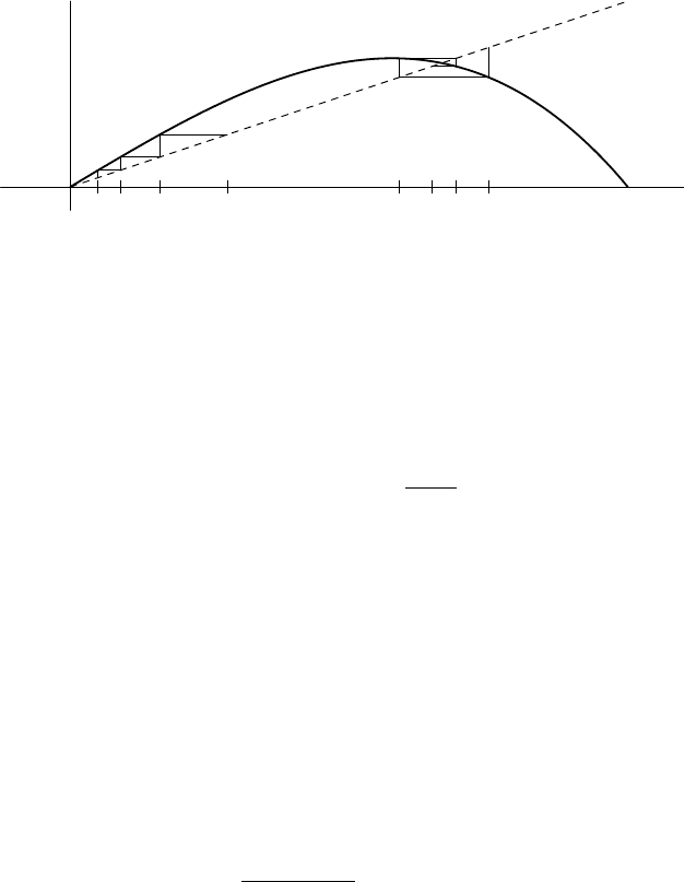
Consider the graph of the function given in Figure 11.2. Fixed points corre-
spond to the intersection of the graph of T with the line y = x. Starting with
any point x
0
, mark the point (x
0
, x
0
) on the diagonal. A vertical line from this
point meets the graph of T at (x
0
, T x
0
) = (x
0
, x
1
). Then a horizontal line from
here meets the diagonal at (x
1
, x
1
). Repeated application yields a graphical pic-
ture of the dynamics. Note that starting near a fixed point, the slope of the graph
determines whether the points approach or move away from the fixed point.
In our example, another typical behaviour is exhibited by all |x| sufficiently
large. For the sake of simplicity, consider |x| > 2. Then
|T x| = 1.8(x
2
− 1)|x| ≥ 5.4|x|.
It is clear then that lim
n→∞
|T
n
x| = +∞. So all of these orbits go off to infinity.
Usually we will try to restrict our domain to a bounded region that is mapped back
into itself by the transformation T .
We now connect our classification of fixed points with derivatives. Say that
T is a C
1
dynamical system on X ⊂ R if the function T is C
1
, that is, has a
continuous derivative.
334 Discrete Dynamical Systems
x
y
y = x
x
0
x
1
x
2
x
3
x
0
x
1
x
2
x
3
FIGURE 11.2. Fixed points for Tx = 1.8(x − x
3
).
.
11.1.2. LEMMA. Suppose that T is a C
1
dynamical system with a fixed point
x
∗
. If |T
0
(x
∗
)| < c < 1, then x
∗
is an attractive fixed point. Moreover, there is an
interval U = (x
∗
− r, x
∗
+ r) about x
∗
so that for every x
0
∈ U, the sequence
x
n
= T
n
x
0
satisfies
|x
n
− x
∗
| ≤ c
n
|x
0
− x
∗
| ≤
c
n
1 − c
|x
1
− x
0
|.
If |T
0
(x
∗
)| > 1, then x
∗
is an repelling fixed point.
PROOF. Suppose that |T
0
(x
∗
)| < c < 1, and let ε = c − |T
0
(x
∗
)| > 0. By the
continuity of T
0
, there is an r > 0 so that
|T
0
(x) − T
0
(x
∗
)| < ε for all x
∗
− r < x < x
∗
+ r.
Hence for x in the interval U = (x
∗
− r, x
∗
+ r),
|T
0
(x)| ≤ |T
0
(x
∗
)| + |T
0
(x) − T
0
(x
∗
)| < (c − ε) + ε = c.
Let x
0
be an arbitrary point in U , and consider the sequence x
n
= T
n
x
0
.
Applying the Mean Value Theorem to the points x
n
and x
∗
, there is a point z
between them so that
T x
n
− T x
∗
x
n
− x
∗
= T
0
(z).
Rewriting this using T x
n
= x
n+1
and T x
∗
= x
∗
, we obtain
|x
n+1
− x
∗
| = |T
0
(z)||x
n
− x
∗
|.
Provided that x
n
belongs to the interval U , we obtain that
|x
n+1
− x
∗
| < c|x
n
− x
∗
|.
In particular, x
n+1
is closer to x
∗
than x
n
is; and therefore x
n+1
also belongs to U.
By induction, we obtain (verify this!) that
|x
n
− x
∗
| < c
n
|x
0
− x
∗
| for all n ≥ 1.
Hence lim
n→∞
|x
n
−x
∗
| = 0 by the Squeeze Theorem. That is, lim
n→∞
x
n
= x
∗
. So x
∗
is an attractive fixed point.
11.1 Fixed Points and the Contraction Principle 335
x
y
y = x
x
∗
(x
0
, x
0
)
(x
1
, x
1
)
(x
2
, x
2
)
(x
3
, x
3
)
(y
0
, y
0
)
(y
1
, y
1
)
(y
2
, y
2
)
(y
3
, y
3
)
x
y
y = x
x
∗
(x
0
, x
0
)
(x
1
, x
1
)
(x
2
, x
2
)
(x
3
, x
3
)
(y
0
, y
0
)
(y
1
, y
1
)
(y
2
, y
2
)
(y
3
, y
3
)
x
y
y = x
x
∗
(x
0
, x
0
)
(x
1
, x
1
)
(x
2
, x
2
)
x
y
y = x
x
∗
(x
1
, x
1
)
(x
2
, x
2
)
(x
3
, x
3
)
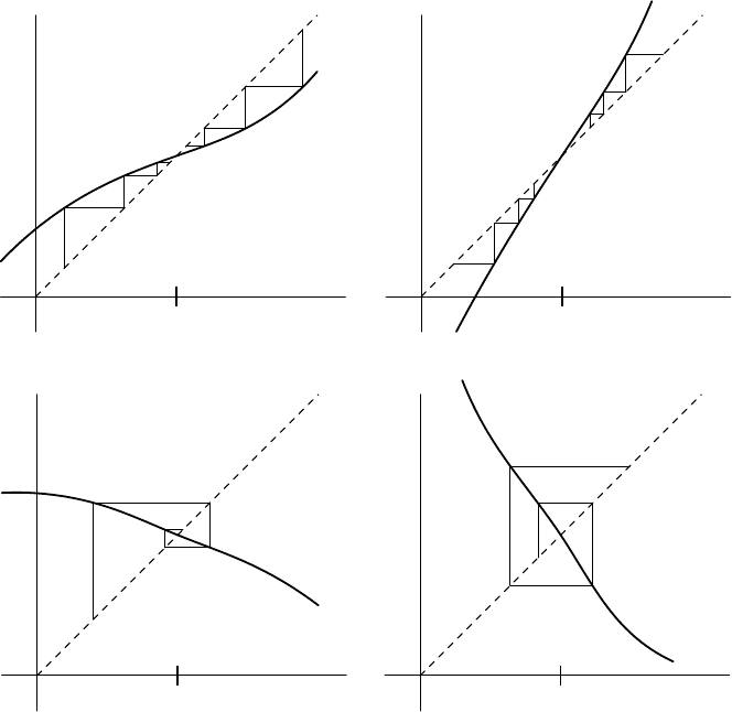
FIGURE 11.3. Iteration of a function g.
Similarly, suppose that |T
0
(x
∗
)| > c > 1, and let ε = |T
0
(x
∗
)|−c > 0. By the
continuity of T
0
, there is an r > 0 so that
|T
0
(x) − T
0
(x
∗
)| < ε for all x
∗
− r < x < x
∗
+ r.
Hence for x in the interval U = (x
∗
− r, x
∗
+ r),
|T
0
(x)| ≥ |T
0
(x
∗
)| − |T
0
(x) − T
0
(x
∗
)| > (c + ε) − ε = c.
The Mean Value Theorem argument works the same way as long as x
n
belongs
to the interval U. However, in this case, repeated iteration eventually moves x
n
outside of U, at which point we have almost no information about the dynamics of
T . So as long as x
n
is in U, we obtain a point z between x
n
and x
∗
so that
|x
n+1
− x
∗
| = |T
0
(z)||x
n
− x
∗
| > c|x
n
− x
∗
|.
This can be repeated as long as x
n
remains inside U to obtain
|x
n
− x
∗
| > c
n
|x
0
− x
∗
|.
As this distance to x
∗
is tending to +∞, repeated iteration eventually will move
x
n+1
outside of U. Therefore, x
∗
is a repelling fixed point. ¥

336 Discrete Dynamical Systems
Notice that in this proof, we only used differentiability in order to apply the
Mean Value Theorem and obtain a distance estimate. The following definition de-
scribes this distance estimate directly, and so allows us to abstract the arguments of
the previous proof to other settings, where differentiability may not hold. However,
we demand that these estimates hold on the whole domain. While this may seem
to be excessively strong, remember that we may be able to restrict our attention to
a smaller domain in which these conditions apply. For example, in our previous
proof, the interval U would be a suitable domain.
11.1.3. DEFINITION. Let X be a subset of a normed vector space (V, k ·k). A
map T : X → X is called a contraction on X if there is a positive constant c < 1
so that
kT x − T yk ≤ ckx − yk for all x, y ∈ X.
That is, T is Lipschitz with constant c < 1.
11.1.4. EXAMPLE. Let us look more closely at the map T x = 1.8(x − x
3
)
introduced in the first section. The fixed points are −
2
3
, 0, and
2
3
.
Now |T
0
(
2
3
)| = | − .6| < 1, so this is an attracting fixed point. We will show
that T is a contraction on the interval [.5, .7]. In this interval, T has a single critical
point at 1/
√
3, a local maximum, and
T (.5) = .675, T (1/
√
3) = .4
√
3 ≈ .6928, and T (.7) = .6426.
As T is increasing on [.5, 1/
√
3] and decreasing on [1/
√
3, .7], it follows that T
maps [.5, .7] into itself. Moreover,
sup
.5≤x≤.7
|T
0
(x)| = sup
.5≤x≤.7
1.8|1 − 3x
2
| = max{|.45|, | − 0.846|} = 0.846.
Therefore, T is a contraction on [.5, .7] with contraction constant c = .846.
Now consider the fixed point 0. Since T
0
(0) = 1.8 > 1, this is a repelling fixed
point. On the interval [−
1
3
,
1
3
], we have
inf
|x|≤
1
3
T
0
(x) = inf
|x|≤
1
3
1.8(1 − 3x
2
) = 1.2.
So the proof of Lemma 11.1.2 shows that
|T x| ≥ 1.2|x| for all x ∈ [−
1
3
,
1
3
].
So the sequence T
n
x moves away from 0 until it leaves this interval.
11.1.5. EXAMPLE. Consider the linear function T (x) = mx + b for x ∈ R.
Then
|T x − T y| = |m||x − y|.
Hence T is a contraction on R provided that |m| < 1. This map has a fixed point if
there is a solution to
x = T x = mx + b.

11.1 Fixed Points and the Contraction Principle 337
It is easy to compute that x
∗
=
b
1−m
is the unique solution provided that m 6= 1.
What happens when m = 1?
We may think of T as the dynamical system on R that maps each point x to
T x. Consider the forward orbit O(x) = {T
n
x : n ≥ 0} of a point x. We obtain a
sequence defined by the recurrence
x
n+1
= T x
n
for n ≥ 0.
A simple calculation shows that
x
1
= mx
0
+ b
x
2
= m
2
x
0
+ (1 + m)b
x
3
= m
3
x
0
+ (1 + m + m
2
)b
x
4
= m
4
x
0
+ (1 + m + m
2
+ m
3
)b.
It appears that there is a general formula
x
n
= m
n
x
0
+ (1 + m + m
2
+ ··· + m
n−1
)b.
We may verify this by induction. It evidently holds true for n = 1. Suppose that it
is valid for a given n. Then
x
n+1
= mx
n
+ b = m
¡
m
n
x
0
+ (1 + m + m
2
+ ··· + m
n−1
)b
¢
+ b
= m
n+1
x
0
+ (m + m
2
+ ··· + m
n
)b + b
= m
n+1
x
0
+ (1 + m + m
2
+ ··· + m
n
)b.
Hence the formula follows for n + 1, and so for all positive integers by induction.
When |m| < 1, the contraction case, this sequence has a limit that we obtain
by summing an infinite geometric series.
lim
n→∞
x
n
= lim
n→∞
m
n
x
0
+ (1 + m + m
2
+ ··· + m
n−1
)b
= 0 + b
∞
X
k=0
m
k
=
b
1 − m
Hence this sequence converges to the fixed point x
∗
. Therefore, x
∗
is an attractive
fixed point that may be located by starting anywhere and iterating T . This means
that an approximate solution to T x = x will be stable, meaning that the orbit of
any point close to x
∗
will remain close to x
∗
. In fact, it was not even necessary to
start close to x
∗
to obtain convergence.
On the other hand, when |m| > 1, lim
n→∞
|x
n
| = ∞ and so this sequence di-
verges. There is still a fixed point, but it is repelling. In this case, the answer is in
the past. The map T is one to one and thus we may solve for
T
−1
x = (x − b)/m =
1
m
x −
b
m
.
This map T
−1
is a contraction, and we can apply the previous analysis to it. Each
point x comes from the point x
−1
= T
−1
x. Going “back into the past” by setting
x
−n−1
= T
−1
x
−n
converges to the fixed point x
∗
. As points close to x
∗
move
outward and eventually go off to infinity, x
∗
is a source.

338 Discrete Dynamical Systems
Finally, when m = −1, there is a unique fixed point. But this point cannot be
located as the limit of an orbit. The reason is that
T
2
x = −(T x) + b = −(−x + b) + b = x.
That is, T
2
equals the identity map on R. So with the exception of the fixed point
x
∗
= b/2, every point has a period 2 orbit.
11.1.6. THE BANACH CONTRACTION PRINCIPLE.
Let X be a closed subset of a complete normed vector space (V, k · k). If T is a
contraction map of X into X, then T has a unique fixed point x
∗
. Furthermore, if
x is any vector in X, then x
∗
= lim
n→∞
T
n
x and
kT
n
x − x
∗
k ≤ c
n
kx − x
∗
k ≤
c
n
1 − c
kx − T xk,
where c is the Lipschitz constant for T .
PROOF. The statement of the theorem suggests how the proof should proceed. Pick
any point x
0
in X and form the sequence (x
n
) given by x
n+1
= T x
n
for n ≥ 0.
CLAIM: This sequence is Cauchy. To see this, first observe that
kx
n+1
− x
n
k = kT x
n
− T x
n−1
k
≤ ckx
n
− x
n−1
k
≤ c
2
kx
n−1
− x
n−2
k
≤ c
n
kx
1
− x
0
k = c
n
D,
where D = kx
1
−x
0
k is a finite number. Using this fact and the triangle inequality,
we compute
kx
n+m
− x
n
k ≤
m−1
X
i=0
kx
n+i+1
− x
n+i
k ≤
m−1
X
i=0
c
n+i
D(11.1.7)
<
∞
X
i=0
c
n+i
D =
c
n
(1 − c)
D.
Given ε > 0, choose N so large that c
N
< ε(1 − c)/D, which is possible since
lim
n→∞
c
n
= 0. Hence for n ≥ N and m ≥ 0, we have kx
n+m
− x
n
k < ε. So the
sequence (x
n
) is Cauchy, as claimed.
Because V is complete, the sequence (x
n
) converges to a point in V , say
lim
n→∞
x
n
= x
∗
.
And since X is closed, this limit point belongs to X. Observe that T is uniformly
continuous because it is Lipschitz (Proposition 5.5.4). Using continuity, we have
T x
∗
= T
³
lim
n→∞
x
n
´
= lim
n→∞
T x
n
= lim
n→∞
x
n+1
= x
∗
.
Hence x
∗
is a fixed point.

11.1 Fixed Points and the Contraction Principle 339
Suppose that y ∈ X is also a fixed point: so T y = y. Then
kx
∗
− yk = kT x
∗
− T yk ≤ ckx
∗
− yk.
Since c < 1, this implies that kx
∗
− yk = 0, whence x
∗
= y. Therefore, x
∗
is the
unique fixed point.
Now using the estimate (11.1.7), we obtain that
kT
n
x
0
− x
∗
k = kT
n
x
0
− T
n
x
∗
k
≤ c
n
kx
0
− x
∗
k
= c
n
lim
m→∞
kx
0
− x
m
k
≤ c
n
(1 − c)
−1
kT x
0
− x
0
k.
Finally, for an arbitrary point x in X, the preceding estimates yield the same
story. Since the fixed point is unique, the limit x
∗
is obtained as the limit of every
orbit independent of the starting point. ¥
11.1.8. EXAMPLE. Let V = R, X = [−1, 1] and T x = cos x. By the Mean
Value Theorem, for any x, y ∈ X, there is a point z between x and y so that
|T x − T y| = |x − y||sin z|.
In particular, |z| < 1. Since sinx is increasing on [−1, 1],
max
|z|≤1
|sinz| = |sin±1| = sin1 < 1.
Thus T is a contraction. To find the fixed point experimentally, type any value
into your calculator and repeatedly hit the
cos button. If your calculator is set for
radians, the sequence will converge rapidly to 0.73908513321516064 . . ..
What happens when you do the same for T x = sin x? It is not a contraction.
Nevertheless, there is a unique fixed point sin0 = 0, and the iterated sequence
converges. But it converges at a painfully slow rate. Try it on your calculator. It is
slow because the derivative at the fixed point is cos0 = 1.
Indeed, the inequality 0 < sinθ < θ for θ in (0, π/2] shows that the only fixed
point in [0, ∞) is x = 0. As sinx is odd, the same is true on (−∞, 0]. The first
iteration x
1
= sinx
0
lies in [−1, 1]; and thereafter this inequality shows that if
0 < x
1
≤ 1, then 0 ≤ x
n+1
< x
n
< 1 for n ≥ 1. Likewise, if −1 ≤ x
1
< 0, then
the sequence x
n
is monotone increasing and bounded above by 0. Hence the limit
exists and must be the unique fixed point of sinx. We can use the Taylor series of
sinx (see Exercise 10.1.D) to show that
|sinx − x| ≤
|x|
3
6
.
Thus if x
0
= .1, it follows that
|x
n
− x
n+1
| ≤
x
3
0
6
= 10
−3
/6.

340 Discrete Dynamical Systems
Since each step moves us at most 10
−3
/6, it will take over
.1 − .01
10
−3
/6
= 540 iter-
ations before x
n
≤ .01. After that, it will take at least 54,000 iterations to get
below .001 and 5.4 million more steps to obtain a fourth decimal of accuracy in the
approximation of the fixed point.
One moral of this example is that for maps T that are not contractions, even if
applying T moves a point x very little, x need not be very close to a fixed point x
∗
.
For contractions, it is true and we have a numerical estimate for kx − x
∗
k in terms
of kT x − xk and the Lipschitz constant.
11.1.9. EXAMPLE. If, in the definition of contraction, the condition is weak-
ened to kT x −T yk ≤ kx −yk, then we cannot conclude that there is a fixed point.
For example, take X = R and T x = x + 1. Clearly, T has no fixed points. But
since kT x − T yk = kx − yk, distance is preserved.
Even the strict inequality kT x − T yk < kx − yk is not sufficient. Consider
X = [1, ∞) and Sx = x + x
−1
. Then
|Sx − Sy| = (x +
1
x
) − (y +
1
y
) = |x − y|(1 −
1
xy
) < |x − y|
for all x, y ≥ 1. However, Sx > x for all x, so S has no fixed point.
11.1.10. REMARK. The first part of Lemma 11.1.2 may be proved as a simple
consequence of the Banach Contraction Principle. Indeed, suppose that T is a C
1
dynamical system with a fixed point x
∗
such that |T
0
(x
∗
)| < c < 1. As before,
use the continuity of T
0
to find an interval I = [x
∗
− r, x
∗
+ r] so that |T
0
(x)| ≤ c
for all x ∈ I. The only difference here is that we are using a closed interval and
a ≤ sign instead of an open interval and strict inequality. Apply the Mean Value
Theorem to any two points x, y in I. For such points, there is a point z between
them so that |T x − T y| = |T
0
(z)||x − y| ≤ c|x − y|.
In particular,
|T x − x
∗
| = |T x − T x
∗
| ≤ c|x − x
∗
| ≤ cr.
Therefore, T maps the interval I into itself, and it is a contraction with contraction
constant c. By the Contraction Principle, we see that x
∗
is the unique fixed point in
I. Moreover, we obtain the desired distance estimates.
11.1.11. EXAMPLE. This example deals with a system of linear equations and
looks for a condition that guarantees an attractive fixed point. Let A =
£
a
ij
¤
be an
n × n matrix, and let b = (b
1
, . . . , b
n
) be a (column) vector in R
n
. Consider the
system of equations
(11.1.12) x = Ax + b.
We will try to analyze this problem by studying the dynamical system given by the
map T : R
n
→ R
n
according to the rule
T x = Ax + b.
A solution to (11.1.12) corresponds to a fixed point of T.
11.1 Fixed Points and the Contraction Principle 341
There are various norms on R
n
, and different norms lead to different criteria
for T to be a contraction. In this example, we will use the max norm,
kxk
∞
= max
1≤i≤n
|x
i
|.
If we think of points in R
n
as real-valued functions on {1, . . . , n}, say x(i) = x
i
for 1 ≤ i ≤ n, then this is the uniform norm on a space of continuous functions.
We will show that T is a contraction on R
n
in this norm if and only if
c := max
1≤i≤n
n
X
j=1
|a
ij
| < 1.
First suppose that c ≥ 1. There is some integer i
0
so that
c =
n
X
j=1
|a
i
0
j
|.
Set x
j
= sign(a
i
0
j
). Then
kx − 0k
∞
= kxk
∞
= max
1≤i≤n
|x
i
| = 1
while
kT x − T 0k
∞
= kAxk
∞
≥ |(Ax)
i
0
|
=
n
X
j=1
a
i
0
j
x
j
=
n
X
j=1
|a
i
0
j
|
= c ≥ 1 = kx − 0k
∞
.
So T is not contractive.
On the other hand, if c < 1, then we compute for x, y ∈ R
n
,
kT x − T yk
∞
= kA(x − y)k
∞
= max
1≤i≤n
¯
¯
n
X
j=1
a
ij
(x
j
− y
j
)
¯
¯
≤ max
1≤i≤n
n
X
j=1
|a
ij
||x
j
− y
j
|
≤
³
max
1≤i≤n
n
X
j=1
|a
ij
|
´³
max
1≤j≤n
|x
j
− y
j
|
´
= ckx − yk
∞
.
So T is a contraction.
Thus by the Banach Contraction Principle, we know that there is a unique so-
lution that can be computed iteratively from any starting point. Choose x
0
= 0.
342 Discrete Dynamical Systems
Then
x
1
= T x
0
= b
x
2
= T x
1
= b + Ab = (I + A)b
x
3
= T x
2
= b + A(b + Ab) = (I + A + A
2
)b.
We will show that
x
n
= (I + A + ··· + A
n−1
)b.
This is evident for n = 0, 1, 2, 3 by the previous calculations. Assume it is true for
some integer n. Then
x
n+1
= T x
n
= b + A(I + A + ··· + A
n−1
)b = (I + A + ··· + A
n
)b.
So the formula is established by induction.
The solution to (11.1.12) is the unique fixed point
x
∗
= lim
n→∞
x
n
= lim
n→∞
(I + A + ··· + A
n−1
)b =
∞
X
k=0
A
k
b.
The important factor that makes this infinite sum convergent is that, because T and
A are contractions,
kA
k
bk
∞
= kA
k
b − A
k
0k ≤ c
k
kb − 0k
∞
= c
k
kbk
∞
.
So this series is dominated by a convergent geometric series and thus converges
by the comparison test. Indeed, the same argument shows that the series
∞
P
k=0
A
k
x
converges for every vector x ∈ R
n
. So the sum C =
∞
P
k=0
A
k
makes sense as a
linear transformation. We note that, in particular, if x is any vector in R
n
, then
lim
n→∞
A
n
x = 0. The solution to our problem is x
∗
= Cb.
We know from linear algebra how to solve the equation x = Ax + b. This
leads to (I − A)x = b. When I − A is invertible, there is a unique solution
x = (I − A)
−1
b. This suggests that our contractive condition (11.1.11) leads to
the conclusion that I − A is invertible with inverse C =
∞
P
k=0
A
k
. To see that this is
the case, compute
(I − A)Cx = lim
n→∞
(I − A)(I + A + ··· + A
n−1
)x
= lim
n→∞
(I + A + ··· + A
n−1
)x − (A + A
2
+ ··· + A
n
)x
= lim
n→∞
x − A
n
x = x.
Therefore, I − A has inverse C.