Davidson K.R., Donsig A.P. Real Analysis with Real Applications

Подождите немного. Документ загружается.

10.7 Expansions Using Chebychev Polynomials 313

Exercises for Section 10.7

A. Verify the following properties of the Chebychev polynomials T

(x).

(a) If m is even, then T

is an even function [i.e., T

(−x) = T

(x)], and if m is odd,

then T

is odd [i.e., T

(−x) = −T

(x)].

(b) Show that every polynomial p of degree n has a unique representation using Cheby-

chev polynomials [i.e., there is a unique choice of constants a

, a

, . . . , a

, so that

p(x) = a

(x) + a

(x) + ··· + a

(x)].

(x)) = T

(x)

(d) (1 −x

(x) − xT

(x) + n

(x) = 0

B. Show by induction that T

(x) =

x +

√

− 1

x −

√

− 1

C. Find a sequence of polynomials that converges uniformly to f (x) = |x|

on [−1, 1].

HINT: f is C

D. Suppose that f ∈ C[−1, 1] has a Chebychev series

∞

n=0

. If

∞

n=0

| < ∞, show

that the Chebychev series converges uniformly to f.

HINT: Study the proof of Theorem 10.7.7.

E. Verify the following expansions in Chebychev polynomials:

(a) |x| =

−

∞

j=1

(−1)

−1

(x)

(b)

√

1 − x

−

∞

j=1

− 1

(x)

HINT: Substitute x = cosθ in computing the coefﬁcients. Apply the previousexercise.

F. Suppose that f ∈ C[−1, 1] has a Chebychev series

∞

n=0

(a) Show that E

(f) ≤

∞

k=n+1

(b) Show that E

n+1

) = 1. HINT: Theorem 10.6.4

(f) − |a

n+1

≤

∞

k=n+2

HINT: Show that E

(f) ≥ E

n+1

−

∞

k=n+2

(d) Show that if lim

n→∞

∞

k=n+1

= 0, then lim

n→∞

(f)

n+1

= 1.

G. Let a

be a sequence of real numbers monotone decreasing to 0. Deﬁne the sequence

of polynomials p

(x) =

k=1

− a

k+1

(x).

(a) Show that this sequence converges uniformly on [−1, 1] to a continuous function

f(x). HINT: Weierstrass M-test

(b) Evaluate (f − p

)

cos(3

−n−1

kπ)

for 0 ≤ k ≤ 3

n+1

(f) = a

n+1

. Conclude that there are continuous functions for which

the optimal sequence of polynomials converges exceedingly slowly.

314 Approximation by Polynomials

10.8. Splines

Splines are smooth piecewise polynomials. They are well adapted to use on

computers, and so they are much used in practical work. Because they are closely

related to polynomials, we give a brief treatment of splines here, concentrating on

issues related to real analysis. For algorithmic and implementation issues, we refer

the reader to [18].

To motivate the idea behind splines, observe that approximation by polyno-

mials can be improved either by increasing the degree of the polynomial or by

decreasing the size of the interval on which the approximation is used. Splines

take the latter approach, successively chopping the interval into small pieces and

approximating the function on each piece by a polynomial of ﬁxed small degree,

such as a cubic.

We search for a relatively smooth function that is piecewise a polynomial of

low degree but is not globally a polynomial at all. This turns out to be worth the ad-

ditional theoretical complications. Why? First, evaluating the approximation will

be easier on each subinterval because it is a polynomial of small degree. Instead of

having to do some multiplications, we have several comparisons to decide which

interval we are in. Comparison is much simpler than multiplication, so evaluation

can be much faster, even if we have to do many comparisons.

Second, since the degree is small, we can use simple methods like interpolation

to ﬁnd the polynomial on each subinterval. Interpolation is both easy to implement

on the computer and (mostly) easy to understand.

Third, local irregularities of the function only affect the approximation locally,

in contrast to polynomial approximation. This means that if a function f is not

differentiable at one point of the interval, then this affects the polynomial approx-

imation over the whole interval. Working with polynomials on subintervals, the

lack of differentiability at one point affects the polynomial approximation on that

subinterval only.

The discussion so far has pretended that we are free to choose completely dif-

ferent polynomials on each subinterval. In fact, we would like the polynomials to

ﬁt together smoothly. To start, we begin with the revealing special case of approxi-

mation by a piecewise linear continuous function.

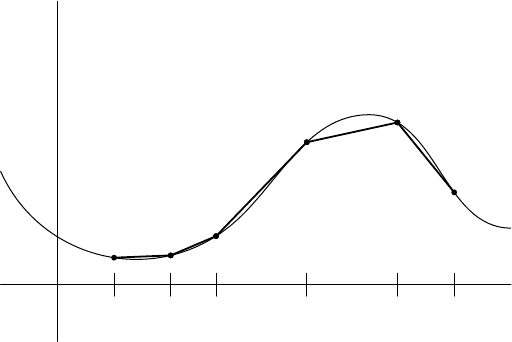
Choose a partition ∆ of the interval [a, b] into k subintervals with endpoints

a = x

< x

< ··· < x

= b. We deﬁne S

(∆) to be the subspace of C[a, b] given

(∆) = {g ∈ C[a, b] : g|

i+1

]

is linear for 0 ≤ i < k}.

Clearly, a function g ∈ S

(∆) is uniquely determined by its values g(x

) at the

nodes x

for 0 ≤ i ≤ k. Indeed, we just construct the line segments between the

points (x

, g(x

)). Thus S

(∆) is a ﬁnite-dimensional subspace of dimension k + 1.

The elements of this space are called linear splines. Figure 10.6 shows an element

of S

(∆) approximating a given continuous function.

Now take a continuous function f in C[a, b]. By Theorem 7.6.5, there is some

g in S

(∆) so that

kf − gk

∞

= inf{kf − hk

∞

: h ∈ S

(∆)}.

10.8 Splines 315

Instead of trying to ﬁnd this optimal choice, we choose the function h in S

(∆) such

that h(x

) = f(x

) for 0 ≤ i ≤ k. Deﬁne J

: C[a, b] → S

(∆) by letting J

f be

this function h. Notice that our characterization of functions in S

(∆) shows that

g = g for g ∈ S

(∆). Also, J

is linear:

(af + bg) = aJ

f + bJ

g for f, g ∈ C[a, b] and a, b ∈ R.

The following lemma shows that choosing J

f instead of the best approximant

does not increase the error too much.

10.8.1. LEMMA. If f ∈ C[a, b], then

kf − J

∞

≤ 2inf{kf − gk

∞

: g ∈ S

(∆)}.

PROOF. Notice that for any f ∈ C[a, b],

∞

= max

|f(x

)| : 0 ≤ i ≤ k

≤ kfk

∞

If g ∈ S

(∆) is the closest point to f , we use linearity and J

g = g to obtain

kf − J

∞

= kf − g − J

(f − g)k

∞

≤ kf − gk

∞

+ kJ

(f − g)k

∞

≤ 2kf − gk

∞

a = x

= b

FIGURE 10.6. Approximation in S

(∆).

10.8.2. DEFINITION. A cubic spline for a partition ∆ of [a, b] is a C

function

h such that h|

i+1

]

a polynomial of degree at most 3 for 0 ≤ i < k. Let S(∆)

denote the vector space of all cubic splines for the partition ∆.

Cubic spline interpolation is popular in practice. It may seem rather surprising

that it is possible to ﬁt cubics together and remain twice continuously differentiable

and still have the ﬂexibility to approximate functions well.

316 Approximation by Polynomials

10.8.3. EXAMPLE. Consider

h(x) =











+ 12x

+ 24x + 16 if − 2 ≤ x ≤ −1

−7x

− 15x

− 3x + 7 if − 1 ≤ x ≤ 0

− 15x

− 3x + 7 if 0 ≤ x ≤ 1

−5x

+ 27x

− 45x + 21 if 1 ≤ x ≤ 2

− 9x

+ 27x − 27 if 2 ≤ x ≤ 3.

We readily compute the following.

(x)

(x) interval

+ 24x + 24 12x + 12 −2 ≤ x ≤ −1

−21x

− 30x − 3 −42x − 15 −1 ≤ x ≤ 0

27x

− 30x − 3 54x − 15 0 ≤ x ≤ 1

−15x

+ 54x − 45 −30x + 27 1 ≤ x ≤ 2

− 18x + 27 6x − 9 2 ≤ x ≤ 3

We can now verify the following table of values.

−2 −1 0 1 2 3

h(x

) 0 2 7 −2 −1 0

) 0 6 −3 −6 3 0

) 0 12 −30 24 −6 0

Since the ﬁrst and second derivative match up at the endpoints of each interval, h

is C

and so is a cubic spline.

To ﬁnd a cubic spline h approximating f, we specify certain conditions. Let us

demand ﬁrst that

h(x

) = f (x

) for 0 ≤ i ≤ k.

Let’s write each cubic polynomial as h

= h|

i+1

]

for 0 ≤ i < k. We need

additional conditions to ensure that h is C

) = h

i+1

), and h

) = h

i+1

) for 1 ≤ i ≤ k − 1.

A cubic has four parameters, and these equations put four conditions on each cubic

exceptfor the two on the ends where there are three constraints. To ﬁnish specifying

the spline, we add two endpoint conditions

) = f

) and h

) = f

assuming that these derivatives exist. (If they do not, we may set them equal to 0.)

For convenience, we shall assume that f is C

, which ensures that these data are

deﬁned and allows some interesting theoretical consequences.

We shall see that a cubic spline h in S(∆) is uniquely determined by these equa-

tions. There are k + 3 data conditions determined by f, namely f(x

), . . . , f(x

)

and f

) and f

). Hence we expect to ﬁnd that S(∆) is a ﬁnite-dimensional

subspace of dimension k + 3. This will allow us to deﬁne a map J from C

[a, b] to

S(∆) by setting Jf to be the function h speciﬁed previously.

10.8 Splines 317

10.8.4. LEMMA. Given c < d and real numbers a

, a

, s

, there is a unique

cubic polynomial p satisfying

p(c) = a

p(d) = a

(d) = s

Setting ∆ = d − c, we obtain

6(a

−a

)

∆

−

+2s

∆

and

(d) = −

6(a

−a

)

∆

+4s

∆

PROOF. Consider the cubics

(x) =

(x − d)

(d − c)

1 + 2

x − c

d − c

(x) =

(x − c)

(d − c)

1 − 2

x − d

d − c

(x) =

(x − c)(x − d)

(d − c)

(x) =

(x − c)

(x − d)

(d − c)

For example, p

(d) = p

(d) = 0. The reader can verify

that p(x) = a

(x) + a

(x) + s

(x) is the desired cubic.

For uniqueness, we can note that the difference of two such cubics is a cubic q

such that q(c) = q(d) = q

(d) = 0. The ﬁrst two conditions show that c

and d are roots of q; and the second two conditions then imply that they are double

roots. So (x − c)

(x − d)

divides q. As q has degree at most 3, this forces q = 0.

Finding the value of p

at c and d is a routine calculation. ¥

10.8.5. THEOREM. Given a partition ∆ : a = x

< x

< ··· < x

= b of the

interval [a, b] and real numbers a

, . . . , a

, s

and s

, there is a unique cubic spline

h ∈ S(∆) such that h(x

) = a

for 0 ≤ i ≤ k and h

(a) = s

and h

(b) = s

PROOF. If such a spline exists, we could deﬁne s

= h

) for 1 ≤ i ≤ k −1. We

search for such values of s

that allow a spline. Given the values a

of h and s

at the points x

i−1

and x

, the previous lemma determines a unique cubic h

the interval [x

i−1

, x

]. So for each choice of (s

, . . . , s

k−1

), there is one piecewise

cubic function on [a, b] that interpolates the values a

and derivatives s

at each

point x

for 0 ≤ i ≤ k. However, in general this will not be C

. There are k − 1

conditions that must be satisﬁed:

) = h

i+1

) for 1 ≤ i ≤ k − 1.

318 Approximation by Polynomials

Our job is to compute a formula for these second derivatives to obtain conditions

on the hypothetical data s

, . . . , s

k−1

Let us write ∆

= x

−x

i−1

for 1 ≤ i ≤ k. By the previous lemma, the second

derivative conditions at x

for 1 ≤ i ≤ k − 1 are

) = −

6(a

− a

i−1

)

∆

i−1

+ 4s

∆

(10.8.6)

6(a

i+1

− a

)

∆

i+1

−

+ 2s

i+1

∆

i+1

Rearranging this yields a linear system of k − 1 equations in the k − 1 unknowns

, . . . , s

k−1

. For 1 ≤ i ≤ k − 1,

∆

i+1

i−1

+ 2(∆

+∆

i+1

+ ∆

i+1

3∆

i+1

−a

)

∆

i+1

3∆

i+1

−a

i−1

)

∆

The terms involving s

and s

may be moved to the right-hand side.

It now remains to show that this system has a unique solution. This will follow

if we can show that the matrix

X =







2(∆

+∆

) ∆

0 0 . . . 0

∆

2(∆

+∆

) ∆

0 . . . 0

0 . . . 0 ∆

k−1

2(∆

k−2

+∆

k−1

) ∆

k−2

0 . . . 0 0 ∆

2(∆

k−1

+∆

)







is invertible. The property of this system that makes it possible is that the matrix is

diagonally dominant, which means that the diagonal entries are greater than the

sum of all other entries in each row.

To see this, suppose that y = (y

, . . . , y

k−1

) is in the kernel of X. Choose a

coefﬁcient i

so that |y

| ≥ |y

| for 1 ≤ j ≤ k − 1. Then looking only at the i

coefﬁcient of 0 = Xy, we obtain

0 =

∆

−1

+ 2(∆

+∆

+ ∆

≥ 2(∆

+∆

)|y

| − ∆

−1

| − ∆

≥ (∆

+∆

)|y

Hence y = 0 and so X has trivial kernel. Hence X is invertible. So for each set of

data a

, . . . , a

, s

and s

, there is a unique choice of points s

, . . . , s

k−1

solving

our system. Thus there is a unique spline h ∈ S(∆) satisfying these data. ¥

Thus if f is a C

function on [a, b], there is a unique cubic spline h such that

h(x

) = a

:= f(x

) for 0 ≤ i ≤ k, h

(a) = s

:= f

(a) and h

(b) = s

:= f

(b).

We denote the function h by Jf. Let us show that J is linear. If f

and f

are

functions in C

[a, b] with h

= Jf

, then h = b

+ b

is a spline such that

h(x

) =

+ b

) =

) + b

)

10.8 Splines 319

and

(a) =

+ b

(a)

= b

(a) + b

(a) =

) + b

(a).

Similarly, this holds at b. By the uniqueness of the spline, it follows that

J(b

+ b

) = b

+ b

= b

+ b

In particular, we may ﬁnd speciﬁc splines c

satisfying

(a) = c

(b) = 0 and c

) =

(

1 if j = i

0 if j 6= i

for 0 ≤ i ≤ k. The linear space S(∆) is spanned by {x, x

, c

: 0 ≤ i ≤ k}. To see

this, let h be the spline with data a

, . . . , a

, s

and s

be given. Let q be the unique

quadratic q(x) = cx + dx

such that q

(a) = s

and q

(b) = s

. Then g = h − q

is a spline with g

(a) = g

(b) = 0. Form the spline

s(x) = q(x) +

i=0

g(x

(x).

It is easy to check that s is another spline with the same data as h. Since this

uniquely determines the spline, h = s has the desired form. This exhibits a speciﬁc

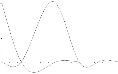
basis for S(∆). Figure 10.7 shows c

and c

for a paricular partition ∆.

2 3

FIGURE 10.7. Graphs of c

and c

for ∆ = {0, .5, 1.4, 2, 2.5, 3}.

Now that we have shown that cubic splines are plentiful, we investigate how

well Jf approximates the original function f . We need the following:

10.8.7. LEMMA. If f ∈ C

[a, b], then for all ϕ ∈ S

(∆),

ϕ(x)(f − Jf)

(x) dx = 0.

320 Approximation by Polynomials

PROOF. We use integration by parts twice. Letting du = (f − Jf )

(x) dx and

v = ϕ(x), we have

ϕ(x)(f − Jf)

(x) dx = ϕ(x)(f − Jf)

(x)

−

(x)(f − Jf)

(x) dx.

Observe that f

(a) = Jf

(a) and f

(b) = Jf

(b), so the ﬁrst term above is zero.

Using integration by parts again with du = (f − Jf)

(x) dx and v = ϕ

(x), the

integral equals

(x)(f − Jf)(x)

−

(x)(f − Jf)(x) dx.

Now, f(a) = Jf(a) and f(b) = Jf(b), so the ﬁrst term is zero. For the second

term, we observe that since ϕ is piecewise linear, ϕ

is equal to zero except for the

points x

, x

, . . . , x

, where it is not deﬁned. Thus the integral is zero. ¥

10.8.8. THEOREM. If f ∈ C

[a, b], then

(x)

dx =

(Jf)

(x)

dx +

(f − Jf)

(x)

dx.

PROOF. Let g = f − Jf. We have

(x)

dx =

(x) + g

(x)

dx + 2

(Jf)

(x)g

(x) dx +

(x)

dx.

However, since Jf ∈ S(∆) is piecewise cubic and C

, it follows that (Jf)

piecewise linear, whence it belongs to S

(∆). Hence by Lemma 10.8.7, the second

term is zero. This gives the required equality, so we’re done. ¥

This allows a characterization of the cubic spline approximating f as optimal

in a certain sense.

10.8.9. COROLLARY. Fix f ∈ C

[a, b]. Among all functions g ∈ C

[a, b] such

that g(x

) = f(x

) for 0 ≤ i ≤ k, g

(a) = f

(a) and g

(b) = f

(b), the cubic

spline interpolant Jf minimizes the energy integral

(x)

dx.

10.8 Splines 321

PROOF. For any such function g, we have Jg = Jf. So by the previous theorem,

(x)

dx =

(Jf)

(x)

dx +

(g − Jf)

(x)

≥

(Jf)

(x)

dx.

This inequality becomes an equality only if g

= (Jf)

. Since we also have

g(a) = Jf(a) and g

(a) = (Jf)

(a) by hypothesis, this implies that g = Jf by

integrating twice. ¥

This property is called the smoothest interpolation property of cubic spline

interpolation. Minimizing

(x) dx is roughly equivalent to minimizing the

strain energy. Historically, ﬂexible thin strips of wood called splines were used

in drafting to approximate curves through a set of points. In 1946, when Schoen-

berg introduced spline curves, he observed that they represent the curves drawn

by means of wooden splines, hence the name. Splines appear to be smooth since

they avoid discontinuous ﬁrst derivatives, which people recognize as “spikes,” and

avoid discontinuous second derivatives, which are recognized as sudden changes in

curvature. Discontinuous third derivatives are not visible in any obvious geometric

way.

Exercises for Section 10.8

A. Fill in the details of the proof of Lemma 10.8.4.

B. Find a nice explicit basis for S

(∆).

C. Show that if f ∈ S

(∆) and f

is continuous on [a, b], then f is a straight line.

D. Show that if f ∈ S(∆) and f

000

is continuous on [a, b], then f is a cubic polynomial.

E. Show that for f ∈ C

[a, b] that kf − Jfk

∞

≤ 2inf{kf − gk

∞

: g ∈ S(∆)}.

HINT: Compare with Lemma 10.8.1.

F. Suppose that ∆ has k > 4 intervals. Let 1 ≤ i ≤ k − 4. If h ∈ S(∆) is 0 everywhere

except on (x

, x

i+3

), show that h = 0. HINT: What derivative conditions are forced?

G. Let x

denote the function max{x

, 0}. Show that every cubic spline in S(∆) has the

form p(x) +

k−1

i=1

(x − x

)

, where p(x) is a cubic polynomial and c

∈ R.

HINT: Given h ∈ S(∆), let c

= δ

/6, where δ

is the change in h

000

at x

H. Find a nonzero spline h for the partition {−1, 0, 1, 2, 3, 4, 5} such that h is 0 on

[−1, 0] ∪ [4, 5]. HINT: Use the previous exercise.

322 Approximation by Polynomials

10.9. Uniform Approximation by Splines

To complete our analysis of cubic splines, we will obtain an estimate for the

error of approximation. This is a rather delicate argument that combines a gener-

alized mean value theorem with another system of linear equations. Our goal is to

establish the following theorem:

10.9.1. THEOREM. Let ∆ be a partition a = x

< x

< ··· < x

= b of the

interval [a, b] and set δ = max{x

− x

i−1

: 1 ≤ i ≤ k}. Let f ∈ C

[a, b] and let

h = Jf be the cubic spline in S(∆) approximating f. Then

kf − hk

∞

≤

ω(f

;δ)

− h

∞

≤ 5δω(f

;δ)

− h

∞

≤ 5ω(f

;δ).

Since the proof is long and computational, we give an overview ﬁrst. Following

the algebra of the last section, we obtain a system of k + 1 linear equations satis-

ﬁed by h

), . . . , h

). The constant terms in this system are estimated using

a second-order Mean Value Theorem. Then the equations are used to show that

) − f

)| ≤ 4ω(f

;δ). It is then straightforward to bound kh

− f

∞

and then integratation gives bounds for kf

− h

∞

and kf − hk

∞

We begin with a second-order Mean Value Theorem.

10.9.2. LEMMA. Suppose that f ∈ C

[a, c] and a < b < c. There is a point ξ

in (a, c) such that

f(b) −

c − b

c − a

f(a) +

b − a

c − a

f(c)

−(c − b)(b − a)

(ξ).

PROOF. Let L(x) be the straight line through (a, f(a)) and (c, f(c)), namely

L(x) =

c − x

c − a

f(a) +

x − a

c − a

f(c).

Consider the function

g(x) = (c − b)(b − a)

f(x) − L(x)

− (c − x)(x − a)

f(b) − L(b)

Notice that g(a) = g(b) = g(c) = 0. So by Rolle’s Theorem, there are points

∈ (a, b) and ξ

∈ (b, c) such that g

(ξ

) = g

(ξ

) = 0. Applying Rolle’s

Theorem to g

now yields a point ξ in (ξ

, ξ

) such that

0 = g

(ξ) = (c − b)(b − a)f

(ξ) + 2

f(b) − L(b)

This is just a rearrangement of the desired formula. ¥

Notice that there is a limiting situation where b equals a or c. Take b = a, for

example. Divide both sides by b−a and take the limit, ignoring the important point