Davidson K.R., Donsig A.P. Real Analysis with Real Applications

Подождите немного. Документ загружается.

10.3 Bernstein’s Proof of the Weierstrass Theorem 293

Now use the positivity of our map B

to obtain

f(x) − f(a)| ≤ B

(x − a)

x − x

− 2ax + a

(x − a)

x − x

Evaluate this at x = a to obtain

f(a) − f(a)| ≤

a − a

≤

2δ

We use the fact that max{a − a

: 0 ≤ a ≤ 1} =

This estimate does not depend on the point a. So we have found

f − fk

∞

≤

2δ

So now choose N ≥

so that

2δ

. Then for all n ≥ N,

f − fk

∞

≤

= ε. ¥

As was already mentioned, using Bernstein polynomials is not an efﬁcient way

of ﬁnding polynomial approximations. However, Bernstein polynomials have other

advantages, which are developed in the Exercises.

Exercises for Section 10.3

A. Show that P

(x) =

(1 − x)

n−k

attains its maximum at

B. Show that kB

∞

≤ kfk

∞

. HINT: Use monotonicity.

C. Prove that B

(f)

≤ B

). HINT: Expand B

((f − a)

D. (a) Compute B

. HINT:

k(k−1)(k−2)+3k(k−1)+k

(b) Compute lim

n→∞

n(B

− x

E. Work through our proof of the Weierstrass theorem with the function f(x) = |x −

on [0, 1] to obtain an estimate for the degree of a polynomial p needed to ensure that

kf − pk

∞

< .0005.

F. (a) Show that B

) = (1 + (e

1/n

− 1)x)

(b) Show that this may be rewritten as (1 +

+ x

)

, where 0 ≤ c

≤ 1.

) converges uniformly to e

on [0, 1].

G. (a) Show that the derivative of B

n+1

f is

n+1

(x) =

k=0

k+1

n+1

− f

n+1

(1 − x)

n−k

(b) If f has a continuous ﬁrst derivative, use the Mean Value Theorem and the uniform

continuity of f to show that lim

n→∞

k(B

− f

∞

= 0.

294 Approximation by Polynomials

H. (a) Fix m ≥ 0 and set f

(x) = x

x −

¢¡

x −

. . .

x −

m−1

for n ≥ 1. Show

that B

= f

(0)x

(b) Hence show that as n tends to inﬁnity, both sequences (f

) and (B

) con-

verge uniformly to x

converges to x

by estimating

− x

∞

≤ kB

− f

∞

+ kB

− x

∞

(d) Use this to give another proof that B

p converges uniformly to p for every polyno-

mial p.

10.4. Accuracy of Approximation

In this section, we try to measure the speed of convergence of polynomial ap-

proximations. Let us deﬁne the best possible error. The aim is to get a reasonable

idea of what it is for a given function, and how well a given approximation com-

pares with it.

Let P

denote the vector space of polynomials of degree at most n. We will

write P

[a, b] to mean that P

is considered as a subspace of C[a, b] with norm

given by the maximum modulus over the interval [a, b].

10.4.1. DEFINITION. If f ∈ C[a, b], then deﬁne the error function E

(f) by

(f) = inf{kf − qk

∞

: q ∈ P

Likewise, if F is a set of functions, we let

(F) = sup

f∈F

(f).

We will know how good a polynomial approximation p ∈ P

to f is by how

close kf − pk

∞

is to E

(f).

A little thought reveals that wildly oscillating functions will not be well approx-

imated by polynomials of low degree. For example, the function f(x) = cos(nπx)

in C[0, 1] alternately takes the extreme values ±1 at

for 0 ≤ k ≤ n. Any function

close to f (within 1) will have to switch signs between these points. This suggests

that in order to get a reasonable estimate, we must measure how quickly f varies.

10.4.2. DEFINITION. The modulus of continuity of f ∈ C[a, b] is deﬁned for

each δ > 0 by

ω(f; δ) = sup

|f(x

) − f (x

)| : |x

− x

| < δ, x

, x

∈ [a, b]

In other words, ω(f, δ) is the smallest choice of ε for which δ “works” in the

deﬁnition of uniform continuity. This is closely related to the notion of oscillation

used in the proof of Lebesgue’s Theorem (Theorem 6.6.6).

10.4 Accuracy of Approximation 295

By Theorem 5.5.9, every continuous function on the compact set [0, 1] is uni-

formly continuous. Therefore, for each ε > 0, there is a δ > 0 such that

|f(x) − f(y)| < ε for all |x − y| < δ, x, y ∈ [0, 1].

Restating this with our new terminology, we see that for every ε > 0, there is a

δ > 0 such that ω(f;δ) < ε. Thus the uniform continuity of f is equivalent to

lim

δ→0

ω(f; δ) = 0.

10.4.3. EXAMPLE. Consider f(x) =

√

x on [0, 1]. Fix δ ≥ 0 and look at

sup

0≤t≤δ

f(x + t) − f (x) =

√

x + δ −

√

x + δ +

√

≤

√

δ.

This inequality is sharp at x = 0. Thus, ω(f ;δ) =

√

δ.

The class of functions f with ω(f;δ) ≤ δ for all δ > 0 are precisely the

functions satisfying

|f(x) − f(y)| ≤ |x − y|,

namely the functions with Lipschitz constant 1. Denote by S the class of functions

in C[0, 1] with Lipschitz constant 1. We will prove our results ﬁrst for the class S.

A good lower bound for the error is obtained using an idea due to Chebychev.

We will use the idea behind the next proof repeatedly, so examine it carefully.

10.4.4. PROPOSITION. E

(S) ≥

2n + 2

for n ≥ 0.

PROOF. Fix n ≥ 0. Consider the sawtoothed function f that takes the values

n+1

(−1)

2n + 2

for 0 ≤ k ≤ n + 1

and is linear in between with slope ±1. Clearly, f belongs to S.

We will show that the closest polynomial to f in P

is the zero polynomial,

which is clearly distance 1/(2n + 2) from f. To this end, suppose that p is a

polynomial with kp − f k

∞

2n+2

. Then

n+1

−

(−1)

2n + 2

It follows that signp

n+1

= (−1)

. Consequently, p changes sign between

n+1

and

k+1

n+1

for each 0 ≤ k ≤ n. By the Intermediate Value Theorem (Theorem 5.6.1),

p has a root in the open interval (

n+1

k+1

n+1

). So p is a nonconstant polynomial with

at least n + 1 roots, and thus is not in P

. Consequently,

(S) ≥ E

(f) = kfk

∞

2n + 2

. ¥

296 Approximation by Polynomials

To obtain an upper bound, let us look carefully at the estimate that comes out

of Bernstein’s proof of the Weierstrass Theorem.

10.4.5. PROPOSITION. If f ∈ C[0, 1] has Lipschitz constant 1, then

f − fk ≤

√

PROOF. We recall the details of the proof of the Weierstrass Approximation The-

orem in our context. Let ε be any positive number. We claim that the Lipschitz

condition gives the strong inequality

|f(x) − f(a)| ≤ |x − a| ≤ ε +

(x − a)

To check this, consider the cases |x − a| ≤ ε and |x − a| > ε separately.

Now apply the Bernstein map B

, which by monotonicity yields

f(x) − f(a)| ≤ ε +

(x − a)

= ε +

(x − a)

x − x

nε

Substituting x = a and maximizing over [0, 1], we obtain

f − fk

∞

≤ ε +

nε

kx − x

∞

= ε +

4nε

Minimizing this leads to the choice of ε =

√

. Thus

f − fk

∞

≤

√

There is quite a gap between our upper and lower bounds when n is large. In

fact, the lower bound has the correct order of growth. In order to obtain superior

upper bounds, we need to replace Bernstein approximations B

f with a better

method of polynomial approximation. We do this in Section 14.9 using Fourier

series.

Exercises for Section 10.4

A. Show that ω(f ; δ

) ≤ ω(f;δ

) if δ

≤ δ

B. If f is C

on [a, b], show that ω(f;δ) ≤ kf

∞

δ.

C. Show that a function f on R is uniformly continuous if and only if lim

δ→0

ω(f;δ) = 0.

D. Show that f is Lipschitz with constant L if and only if f satisﬁes ω(f, δ) ≤ Lδ.

E. If f is Lipschitz with constant L, prove that kB

f − fk ≤

√

F. For f, g ∈ C[a, b] and α, β ∈ R,

(a) Show that E

(αf + βg) ≤ |α|E

(f) + |β|E

(g).

(b) Show that E

m+n

(fg) ≤ kfk

∞

(g) + kgk

∞

(f).

G. Show that if lim

δ→0

ω(f;δ)

= 0, then f is constant.

10.5 Existence of Best Approximations 297

H. (a) In C[0, 1], show that E

(cosmπx) = 1 for n < m.

(b) Use the Taylor series about a = 1/2 to show that E

10n

(cosnπx) < 10

−3n

I. Let f(x) = |2x − 1| on [0, 1].

(a) Show that B

) = 2

−2n

(b) Compute lim

n→∞

√

. HINT: Use Stirling’s formula (6.5.2).

10.5. Existence of Best Approximations

Suppose that f is a continuous function on [a, b]. We may search for the op-

timal polynomial approximation of given degree. The analysis tools that we have

developed will allow us to show that such an optimal approximation always exists.

Moreover, in the next section, the best approximation will be shown to be unique.

A polynomial p(x) = a

+ a

x + ···+ a

of degree at most n is determined

by the n + 1 coefﬁcients a

, . . . , a

. Moreover, a nonzero polynomial of this form

has at most n zeros and thus is not equal to the zero function on [a, b]. Hence

[a, b] is an (n + 1)-dimensional vector subspace of C[a, b]. It may be identiﬁed

with R

n+1

by associating p to the vector (a

, . . . , a

). The norm is quite different

from the Euclidean norm. However, the results of Section 7.6 are precisely what

we need to solve our problem.

First, Lemma 7.6.1 shows that there are constants 0 < c < C (depending on

a, b and n) such that every polynomial p(x) = a

+ a

x + ··· + a

in P

[a, b]

satisﬁes

k=0

1/2

≤ kpk

∞

= sup

a≤x≤b

|p(x)| ≤ C

k=0

1/2

This lemma allows us to transfer our convergence results for R

n+1

over to P

It is important to note that these results depend on having a ﬁxed bound on the

degree of the polynomials. They are false for polynomials of unbounded degree.

10.5.1. COROLLARY. P

[a, b] has the same convergent sequences as R

n+1

the sense that sequence p

k=0

in P

[a, b] converges uniformly on [a, b] to

a polynomial p =

k=0

if and only if lim

i→∞

= a

for 0 ≤ k ≤ n.

PROOF. Let p

correspond to the vector a

= (a

, . . . , a

) for i ≥ 1, and let p

correspond to the vector a. Then if a

converges a, then

lim

i→∞

kp − p

∞

≤ lim

i→∞

Cka − a

= 0.

298 Approximation by Polynomials

Hence p

converges uniformly to p on [a, b]. Conversely, if p

converges uniformly

to p on [a, b], then

lim

i→∞

ka − a

≤ lim

i→∞

kp − p

∞

= 0.

So a

converges to a in the Euclidean norm.

The second statement follows from Lemma 4.2.3, which shows that a sequence

converges in R

n+1

if and only if each coefﬁcient converges. ¥

Second, Corollary 7.6.3 applies directly. Again this is false if the degree of the

polynomials is not bounded.

10.5.2. COROLLARY. A subset of P

[a, b] is compact if and only if it is closed

and bounded.

Finally, an immediate consequence of Theorem 7.6.5 is the result we are look-

ing for.

10.5.3. THEOREM. Let f be a continuous function on [a, b]. For each integer

n ≥ 0, there exists a closest polynomial of degree at most n to f in the max norm

on C[a, b].

We consider an example that shows that a best approximation in certain more

general circumstances may not exist; and when it does exist, it may not be unique.

10.5.4. EXAMPLE. Consider the subspace

S = {h ∈ C[0, 1] : h(0) = 0}

of C[0, 1]. Note that if f is any function in C[0, 1], then f − f(0) belongs to S.

This shows that the linear span of S and the constant function 1 is all of C[0, 1]. We

therefore say that S is a subspace of codimension one. In particular, it is inﬁnite-

dimensional since C[0, 1] is inﬁnite dimensional. So the type of arguments we used

for P

do not apply.

Consider the function f = 1. What are the best approximations to f in S?

Clearly, for any h ∈ S,

kf − hk

∞

≥ |f(0) − h(0)| = 1.

On the other hand, kf − hk

∞

= 1 is equivalent to the inequalities

0 ≤ h(x) ≤ 2 for all 0 ≤ x ≤ 1.

There are many functions h ∈ S within these constraints. For example, h

= 0,

(x) = x/2, h

(x) = 2x, and h

(x) =

sin

(6πx). We see that there are

(inﬁnitely) many closest points.

Now consider the subspace

T = {h ∈ S :

h(x) dx = 0}.

10.5 Existence of Best Approximations 299

This is a subspace because if g and h belong to T and α and β are in R, then

(αg + βh)(0) = 0 and

(αg + βh)(x) dx = α

g(x) dx + β

h(x) dx = 0.

The subspace T has codimension 2 because C[0, 1] is spanned by T , 1 and x.

Moreover, it is closed. For if h

∈ T converge uniformly to a function h, then h(0)

equals the limit of h

(0), which is 0, and by Theorem 8.3.1,

h(x) dx = lim

n→∞

(x) dx = 0.

So h belongs to T .

Let g(x) = x and consider the distance of g to T . Note that g(0) = 0 but

g(x) dx =

Suppose that h ∈ T , and compute that

g(x) − h(x) dx ≤

kg − hk

∞

dx = kg − hk

∞

If kg − hk

∞

, then this inequality must be an equality. This can only occur if

g(x) − h(x) = kg − hk

∞

for all 0 ≤ x ≤ 1.

This implies that h(x) = x −

. Note that h does not lie in T because h(0) 6= 0.

So the distance 1/2 is not attained.

However, we can easily come arbitrarily close to this distance. Indeed, we will

show that for any integer n, there will be a continuous function h

in T so that

kg −h

∞

. The idea is to make h

(x) = x −

−

on [a

, 1], h

(0) = 0

and linear in between, with a

chosen so that the integral is zero. It is easy to

check that the function with these properties does the job. A calculation shows that

n+2

. We ﬁnd

(x) =











−

(n − 2)

x for 0 ≤ x ≤

n + 2

x −

−

for

n + 2

≤ x ≤ 1.

This shows that when inﬁnite-dimensional subspaces are involved, there need

not be a closest point.

Exercises for Section 10.5

A. Suppose that f ∈ C[0, 1] satisﬁes f(0) = f(1) = 0.

(a) Show that f is a limit of polynomials such that p(0) = p(1) = 0.

(b) Show that there is a closest polynomial of degree at most n with this property.

300 Approximation by Polynomials

B. Let f ∈ C

[0, 1]. Show that there is a closest polynomial of degree at most n to f in

the C

[0, 1] norm, analogous to the C

[a, b] norm deﬁned in Example 7.1.4.

C. Find all closest lines p(x) = ax + b to f(x) = x

in the C

[0, 1] norm. Note that the

best approximation is not unique.

D. Find the closest polynomial to sinx on R.

E. (a) Show that for every bounded function on [a, b], there is aclosest polynomial p ∈ P

in the max norm.

(b) Show by example that a closest polynomial need not be unique.

F. Recall that a norm is strictly convex if kxk = kyk = k(x + y)/2k implies that x = y.

(a) Suppose that V has a strictly convex norm and M is a ﬁnite-dimensional subspace

of V . Prove that each v ∈ V has a unique closest point in M.

(b) Prove that an inner product norm is strictly convex.

10.6. Characterizing Best Approximations

Perhaps in view of the previous examples, it is surprising that the best polyno-

mial approximant of degree n to any continuous function f is uniquely determined.

However, it is unique. We are able to show this because there is an interesting

condition that characterizes this best approximation. This result was established by

Borel in 1905, building on work of Chebychev.

10.6.1. EXAMPLE. Consider any continuous function f in C[0, 1]. What is the

best approximation by a polynomial of degree 0 (i.e., a constant)? We want to make

kf − ck

∞

is as small as possible. By the Extreme Value Theorem, there are two

points x

min

and x

max

in [0, 1] so that

f(x

min

) ≤ f (x) ≤ f(x

max

) for all 0 ≤ x ≤ 1.

Clearly, kf − ck

∞

is the maximum of |f(x

min

) − c| and |f(x

max

) − c|. To make

both as small as possible, we must take

c =

f(x

min

) + f(x

max

)

With this choice, the error r(x) = f(x) − c satisﬁes

r(x

max

) = krk

∞

f(x

max

) − f (x

min

)

and

r(x

min

) = −krk

∞

= −

f(x

max

) − f (x

min

)

10.6.2. EXAMPLE. Consider the continuous function f(x) = x

in C[0, 1].

What is the best linear approximation? One approach is to ﬁnd the maximum mod-

ulus of x

− ax − b and then minimize over choices of a and b. This is a calculus

10.6 Characterizing Best Approximations 301

problem that is not too difﬁcult. However, our approach will be to “guess” the

answer and to verify it by geometric means.

First subtract x from f to get g(x) = x

−x. This function is symmetric about

the line x =

. It takes its maximum value 0 at both 0 and 1, while its minimum is

−

at x =

. From the previous example, we know that to minimize kg(x) − bk

∞

we should set the constant b equal to −

so that the maximum and minima have the

same absolute value,

. This intuitive approach yields a guess that the best linear

approximation is x −

. The error is r(x) = x

− x +

. We know that

r(0) =

, r(

) = −

, and r(1) =

Now we will show that y = x −

is indeed the closest line to x

on [0, 1].

Equivalently, it sufﬁces to show that y = 0 is the closest line to y = r(x) on [0, 1].

Suppose that some linear function g satisﬁes kr − gk <

. Then

g(0) ∈ (0,

), g(

) ∈ (−

, 0), and g(1) ∈ (0,

Therefore,

g(0) > 0 > g(

) < 0 < g(1).

By the Intermediate Value Theorem, g has a zero between 0 and

and another zero

between

and 1. But g is linear, and thus it has at most one root. This contradiction

shows that no better linear approximation exists.

Notice that the strategy we used in this example is essentially the same as that

used in proving Proposition 10.4.4.

In the ﬁrst example, the best approximation yields an error function r that

achieves the values ±krk

∞

. In the case of our linear approximation, we found

three points at which r alternately achieved the values ±krk

∞

. This notion gener-

alizes to give a condition that is sufﬁcient to be the best approximation.

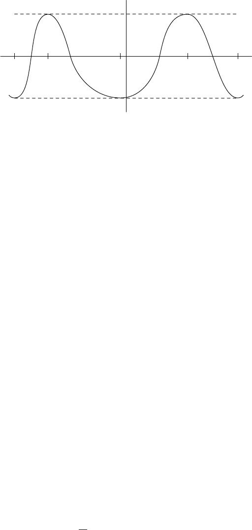
10.6.3. DEFINITION. We say a function g ∈ C[a, b] satisﬁes the equioscilla-

tion condition of degree n if there are n + 2 points x

< x

< ··· < x

n+2

in [a, b]

so that either

g(x

) = (−1)

kgk

∞

for 1 ≤ i ≤ n + 2

g(x

) = (−1)

i+1

kgk

∞

for 1 ≤ i ≤ n + 2.

In other words, g attains its maximum absolute value at n+2 points and it alternates

in sign between these points.

Figure 10.4 shows a function that satisﬁes the equioscillation condition.

10.6.4. THEOREM. Suppose f ∈ C[a, b] and p ∈ P

. If r = f −p satisﬁes the

equioscillation condition of degree n, then

kf − pk

∞

= inf{kf − qk

∞

: q ∈ P

302 Approximation by Polynomials

FIGURE 10.4. A function satisfying the equioscillation condition

PROOF. If the equality were not true, then there would be some nonzero q ∈ P

that p + q is a better approximation to f; that is,

kf − (p + q)k

∞

< kf − pk

∞

or, equivalently,

kr − qk

∞

< krk

∞

In particular, if x

, . . . , x

n+2

are the points from the equioscillation condition for

r, then

|r(x

) − q(x

)| < krk

∞

= |r(x

)| for 1 ≤ i ≤ n + 2.

It follows that q(x

) 6= 0 and has the same sign as r(x

) for 1 ≤ i ≤ n + 2.

Therefore, q changes sign between x

and x

i+1

for 1 ≤ i ≤ n + 1. By the

Intermediate Value Theorem, q has a root between x

and x

i+1

for 1 ≤ i ≤ n + 1.

Hence it has at least n + 1 zeros. But q is a polynomial of degree at most n, so the

only way it can have n + 1 zeros is if q is the zero polynomial. This is false, and

thus no better approximation exists. ¥

The important insight of Chebychev and Borel is that this condition is not only

sufﬁcient, it is also necessary. The argument is more subtle. When the function

r fails to satisfy the equioscillation condition, a better approximation of degree n

needs to be found.

10.6.5. THEOREM. If f ∈ C[a, b] and p ∈ P

satisfy

kf − pk

∞

= inf{kf − qk

∞

: q ∈ P

then f − p satisﬁes the equioscillation condition of degree n.

PROOF. Let r = f − p ∈ C[a, b] and set R = krk

∞

. By Theorem 5.5.9, r is

uniformly continuous on [a, b]. Thus there is a δ > 0 so that

|r(x) − r(y)| <

for all |x − y| < δ, x, y ∈ [a, b].

Partition [a, b] into disjoint intervals of length at most δ. Let I

, I

, . . . , I

denote

those intervals of the partition on which |r(x)| attains the value R (including at the