Cotton W.R., Pielke R.A. Human Impacts on Weather and Climate

Summary of the status of the hypothesis 219

radiation physics. It has also brought to the forefront a realization of the many

potential ecological consequences of climate change and nuclear war.

It is clear that nuclear winter was largely politically motivated from the begin-

ning, and it is an example of science being subverted to political ends. This is not

the way that good science should be conducted.

Global effects of land-use/land-cover change and

vegetation dynamics

11.1 Land-use/land-cover changes

Estimates of the Earth’s landscape which have been disturbed from their natural

state vary according to how the disturbance is defined. In terms of global cultivated

land, Dudal (1987) indicates that 146 ×10

of a potential cultivated coverage

of 3031 × 10

are presently being utilized. Since the Earth’s land surface

covers 13392 × 10

, this indicates that 10.9% of the landscape is cultivated,

with the potential level reaching 22.6% coverage.

This value of land disturbance due to human activities is an underestimate,

however. Brasseur et al. (2005) report that up to half of the Earth’s landscape has

been directly altered. Human activities also include domestic grazing of semi-arid

regions, urbanization, drainage of wetlands, and alterations in species composition

due to the introduction of exotic trees and grasses. In the United States, for

example, 426 000 km

(4.2% of the total land area) have been artificially drained

(Richards, 1986).

In China, of the 2 × 10

in the temperate arid and semi-arid grassland

regions, hundreds of thousands of square kilometers have been degraded due

to overgrazing and the overextension of agriculture, often to the extent that

desertification has occurred (Committee on Scholarly Communication with the

People’s Republic of China, 1992).

The influence of vegetation on climate includes its influence on albedo, water-

holding capacity of the soil, stomatal resistance to water vapor transfer, aero-

dynamic roughness of the surface, and effect on snow cover. These effects are

seasonally varying and are essential in GCM simulations of the effect of vegetation

removal on climate change (Rind, 1984).

The sensitivity of global climate to even small changes in surface properties

has been discussed in Pielke (1991). As described in that paper, an increase of the

average albedo of the land surface of the Earth as viewed from space of 4% would

result in a lowering of the Earth’s equilibrium temperature by 24



C. A decrease

220

Historical land-use change 221

of this average albedo by 4% would increase the equilibrium temperature by

24



C. This is on the same order as the estimates of a global surface equilibrium

temperature change in GCM doubled carbon dioxide radiative–convective model

calculations of 05



C to around 4



The simple analysis presented in Pielke (1991) ignores, of course, how such a

temperature change would be distributed with height or geographically. Nonethe-

less even if the change of equilibrium temperature is reduced by one-half as a

result of these effects, the importance of the landscape energy budget to global

climate is obvious.

There have been almost no global quantitative evaluations of changes in the

heat and moisture fluxes at the surface due to human activity. One pioneering

work that has been completed in this area is Otterman (1977) who estimated the

change in the Earth’s surface albedo over the last few thousand years due to

overgrazing. He has concluded that overgrazing results in a higher albedo of the

trampled, crumbled soil than in the original steppe where there was dark plant

debris accumulating on a crusted soil surface (also see Chapter 6 for a discussion

of overgrazing). Otterman estimated that the current Earth’s surface albedo is

0.154 whereas before anthropogenically caused grazing (6000 years before the

present), this albedo value was 0.141. This albedo change could have resulted

in an average cooling effect of 077



C in the Earth’s equilibrium temperature.

Hartmann (1984) suggested that a shift of precipitation between land and ocean

areas at low latitude can also lead to planetary albedo changes as a result of

alterations in vegetation and through changes in cloud cover distribution resulting

from these changes in land surface albedo. He concluded that this albedo change

could result in an approximately 5



C global mean temperature change without

any other feedbacks. Gordon et al. (2005) have concluded that deforestation

and irrigation have significantly altered atmospheric water vapor flows on a

global scale.

11.2 Historical land-use change

A documentation of global patterns of land-use change from 1700 to 2000 is

presented in Klein Goldewijk (2001). Klein Goldewijk reports on worldwide

changes of land to crops of 136 Mha, 412 Mha, and 658 Mha in the periods

1700-1799, 1800-1899, and 1900-1990, respectively. Conversion to pasture was

418 Mha, 1013 Mha, and 1496 Mha in these three time periods. Figure 11.1

illustrates these changes, including an acceleration of tropical deforestation during

the twentieth century. O’Brien (2000) also documents land-use change for recent

years (Table 11.1).

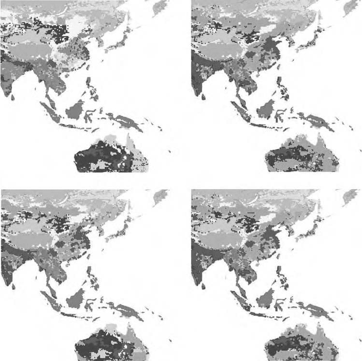
222 Global effects of vegetation dynamics

(a) (c)

(b) (d)

(d) 1990. The human-disturbed landscape includes intensive cropland (red), and

marginal cropland used for grazing (pink). Other landscape includes, for example,

tropical evergreen and deciduous forest (dark green), savanna (light green),

grassland and steppe (yellow), open shrubland (maroon), temperate deciduous

forest (blue), temperate needleleaf evergreen forest (light yellow), and hot desert

(orange). Of particular importance is the expansion of the cropland and grazed

land between 1700 and 1900. Data obtained from the Hyde Database available

at www.mnp.nl/hyde/. Reproduced with permission from Kees Klein Goldewijk.

See also color plate.

Apart from their role as reservoirs, sinks, and sources of carbon, tropical

forests provide numerous additional ecosystem services. Many of these ecosystem

services directly or indirectly influence climate. The climate-related ecosystem

Historical land-use change 223

Table 11.1 Tropical forest extent and loss (rain forest and moist deciduous

forest ecosystems)

Rain forest Moist deciduous forest

Country

Extent in

1990 (kha)

Decrease

1981–90 (%)

Extent in

1990 (kha)

Decrease

1981–90 (%)

Brazil 291 597 6 197 082 16

Indonesia 93 827 20 3 366 20

Democratic Republic of the

Congo (Zaire)

60 437 12 45 209 12

Columbia 47 455 6 4 101 38

Peru 40 358 6 12 299 6

Papua New Guinea 29 323 36 705 6

Venezuela 19 602 14 15 465 36

Malaysia 16 339 36 0 0

Myanmar 12 094 24 10 427 28

Guyana 11 671 0 5 078 6

Suriname 9 042 0 5 726 4

India 8 246 12 7 042 10

Cameroon 8 021 8 9 892 12

French Guiana 7 993 0 3 0

Congo 7 667 4 12 198 4

Ecuador 7 150 34 1 669 34

People’s Democratic

Republic of Laos

3 960 18 4 542 18

Philippines 3 728 62 1 413 54

Thailand 3 082 66 5 232 54

Vietnam 2 894 28 3 382 28

Guatemala 2 542 32 731 0

Mexico 2 441 20 11 110 30

Belize 1 741 0 238 0

Cambodia 1 689 20 3 610 20

Gabon 1 155 12 17 080 12

Central African Republic 616 14 28 357 8

Cuba 114 18 1 247 18

Bolivia 0 0 35 582 22

Source: World Resources Institute (1994), adapted from O’Brien (2000); from Pielke

et al. (2002).

services that tropical forests provide include the maintenance of elevated soil

moisture and surface air humidity, reduced sunlight penetration, weaker near-

surface winds, and the inhibition of anaerobic soil conditions. Such an environment

maintains the productivity of tropical ecosystems (Betts, 1999) and has helped

sustain the rich biodiversity of tropical forests.

224 Global effects of vegetation dynamics

0.8

0.6

0.4

0.2

0.1

–150° –120° –90° –60°

–60° –30° 30° 60°0°

–30° 0° 30° 60° 90° 120° 150°

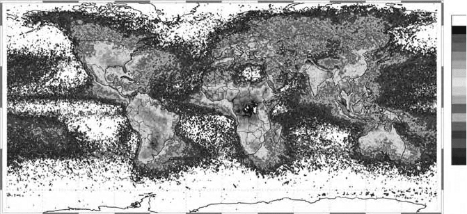
Figure 11.2 Global distribution of lightning from April 1995 through February

2003 from the combined observations of the NASA Optical Transient Detec-

tor (OTD) (4/95-3/00) and Lightning Imaging Sensor (LIS) (1/98-2/03) instru-

ments. From http://thunder.nsstc.nasa.gov/images/HRFC_AnnualFlashRate_cap.

jpg. See also color plate.

11.3 Global perspective

The effect of well above average ocean temperatures in the eastern and central

Pacific Ocean, which is referred to as El Niño, has been shown to have a major

effect on weather, thousands of kilometers from this region (Shabbar et al., 1997).

The presence of the warm ocean surface conditions permits thunderstorms to

occur there that would not have happened with the average colder ocean surface.

These thunderstorms export vast amounts of heat, moisture, and kinetic energy

to the middle and higher latitudes, particularly in the winter hemisphere. This

transfer alters the ridge and trough pattern associated with the polar jet stream

(Hou, 1998). This transfer of heat, moisture, and kinetic energy is referred to as

“teleconnection” (Namias, 1978; Wallace and Gutzler, 1981; Glantz et al., 1991).

Almost two-thirds of the global precipitation occurs associated with mesoscale

cumulonimbus and stratiform cloud systems located equatorward of 30



(Keenan

et al., 1994). In addition, much of the world’s lightning occurs over tropical

land masses, with maxima also over the midlatitude land masses in the warm

seasons (Lyons, 1999; Rosenfeld, 2000) (Fig. 11.2). These tropical regions are

also undergoing rapid landscape change as reported in Section 11.2.

As shown in the pioneering study by Riehl and Malkus (1958), and Riehl

and Simpson (1979), 1500 to 5000 thunderstorms (which they refer to as “hot

towers”) are the conduit to transport this heat, moisture, and wind energy to higher

latitudes. Since thunderstorms only occur in a relatively small percentage of the

Global perspective 225

area of the tropics, a change in their spatial patterns would be expected to have

global climate consequences.

Wu and Newell (1998) concluded that SST variations in the tropical eastern

Pacific Ocean have three unique properties that allow this region to influence the

atmosphere effectively: large magnitude, long persistence, and spatial coherence.

Since land-use change has the same three attributes, a similar teleconnection would

be expected with respect to landscape patterns in the tropics. Dirmeyer and Shukla

(1996), for example, found that doubling the size of deserts in a GCM model

caused alterations in the polar jet stream pattern over northern Europe. Kleidon

et al. (2000) ran a GCM with a “desert world” and a “green planet” in order to

investigate the maximum effect of landscape change. However, these experiments,

while useful, do not represent the actual effect of realistic anthropogenic land-use

change. Actual documented land-use changes are reported, for example, in Baron

et al. (1998), Giambelluca et al. (1999), Leemans (1999), and O’Brien (1997,

2000). Giambelluca et al., for example, report albedo increases in the dry season

of from 0.01 to 0.04 due to deforestation over northern Thailand.

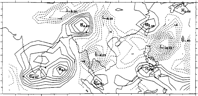
Figure 11.3 illustrates how precipitation patterns in the tropics are altered in

Southeast Asia and adjacent regions in a GCM. Two 10-year simulations were

performed: one with the current global seasonally varying leaf area index and

one with the potential seasonally varying leaf area index, as estimated by Nemani

70° 80° 90° 100° 110° 120° 130° 140°

35°

30°

25°

15°

10°

20°

5°

0°

Figure 11.3 Illustration of how precipitation patterns in the tropics are altered

in Southeast Asia and adjacent regions in a GCM where two 10-year simulations

were performed: one with the current global LAI and one with the potential LAI,

can Geophysical Union. Reproduced by permission of the American Geophysical

Union.

226 Global effects of vegetation dynamics

et al. (1996). No other landscape attributes were changed. The figure presents the

10-year averaged difference in precipitation for the month of July for the two GCM

sensitivity experiments, which illustrates major pattern shifts in precipitation.

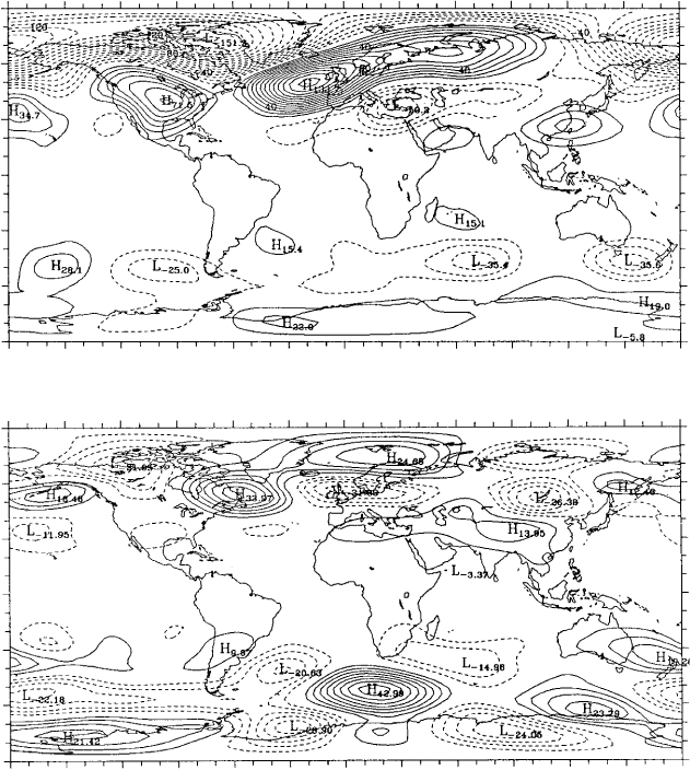
As with El Niño, this alteration in tropical thunderstorm patterning teleconnects

to higher latitudes (Fig. 11.4), where the 10-year averaged 500 mb heights for

July are presented; the 10-year averaged 500 mb heights are also shown for

January.

150°180° 120° 90° 60° 90°60°30°0°30° 120° 150° 180°

90°

(a)

(b)

30°

60°

0°

90°S

150

°180° 120° 90° 60° 90°60°30°0°30° 120° 150° 180°

90°

60°

30°

60°

90°

W E

Figure 11.4 Ten-year averaged differences in 500 mb heights zonal wavenum-

bers 1–6 only (actual LAI minus potential LAI). (a) January, contour 10 m, and

Union. Reproduced by permission of the American Geophysical Union.

Global perspective 227

The GCM produced a major, persistent change in the trough/ridge pattern

of the polar jet stream, most pronounced in the winter hemisphere, which is a

direct result of the land-use change. Unlike an El Niño, however, where cool

ocean temperatures return so that the El Niño effect can be clearly seen in the

synoptic weather data, the landscape change is permanent. Figure 11.5 shows

how the 10-year averaged surface air temperatures changed globally in this model

experiment (Chase et al., 1996).

150°180° 120° 90° 60° 90°60°30°0°30° 120° 150° 180°

90°

(a)

(b)

30°

60°

0°

90°

150°180° 120° 90° 60° 90°60°30°0°30° 120° 150° 180°

90°

60°

30°

60°

0°

90°

W E

Figure 11.5 Ten-year averaged differences in 1.5 m air temperature (actual LAI

minus potential LAI) in K for (a) January, and (b) July. Contour interval is 0.5

by permission of the American Geophysical Union.

228 Global effects of vegetation dynamics

That landscape change in the tropics affects cumulus convection and long-

term precipitation averages should not be a surprising result. For example, as

reported in Pielke et al. (1999b), using identical observed meteorology for lateral

boundary conditions, the Regional Atmospheric Modeling System was integrated

for July–August 1973 for south Florida. Three experiments were performed: one

using the observed 1973 landscape, another the 1993 landscape, and the third the

1900 landscape, when the region was close to its natural state. Over the 2-month

period, there was a 9% decrease in rainfall averaged over south Florida with the

1973 landscape and an 11% decrease with the 1993 landscape, as compared with

the model results when the 1900 landscape is used. A follow-on study further

confirmed these results (Marshall et al., 2004a). The limited available observations

of trends in summer rainfall over this region are consistent with these trends.

Chase et al. (2000) completed more general landscape change experiments using

the CCM3 from the NCAR. In this experiment, two 10-year simulations were

performed using current landscape estimates and the potential natural landscape

estimate under current climate. In addition to LAI differences, albedo, fractional

vegetation coverage, and aerodynamic roughness differences were included. While

the amplitude of the effect of land-use change on the atmospheric response was

less than when the CCM2 GCM model was used, substantial alterations of the

trough/ridge polar jet stream still resulted. Figures 11.6, 11.7, and 11.8 show the

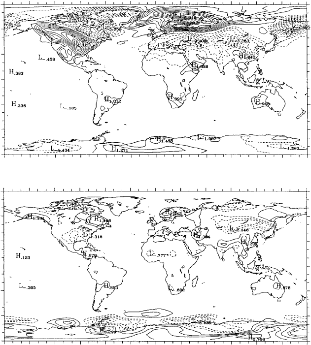
January 10-year averaged cumulus convective precipitation, 200 mb height, and

near-surface temperature differences between the two experiments. Despite the

difference between the experiments with CCM2 and CCM3, both experiments

produce a wavenumber three change pattern in the polar jet stream. Pitman and

Zhao (2000) and Zhao et al. (2001a) have recently performed similar GCM

experiments that have provided confirmation of the Chase et al. (1996, 2000)

results.

Many other studies support the result that there is a significant effect on the

large-scale climate due to land-surface processes (see Table 11.2).

Zeng et al. (1998) found, for example, that the root distribution influences the

latent heat flux over tropical land. Kleidon and Heimann (2000) determined that

deep-rooted vegetation must be adequately represented in order to realistically

represent the tropical climate system. Dirmeyer and Zeng (1999) concluded that

evaporation from the soil surface accounts for a majority of water vapor fluxes

from the surface for all but the most heavily forested areas, where transpiration

dominates. Recycled water vapor from evaporation and transpiration is also a

major component of the continental precipitation. Brubaker et al. (1993) found

that local contributions of water vapor to precipitation generally lie between 10%

to 30%, but can be as high as 40%. Eltahir and Bras (1994a) concluded that

there is 25–35% recycling of precipitation water in the Amazon. Dirmeyer (1999)

Cotton W.R., Pielke R.A. Human Impacts on Weather and Climate

Подождите немного. Документ загружается.