Cohen I.M., Kundu P.K. Fluid Mechanics
Подождите немного. Документ загружается.


802 Introduction to Biofluid Mechanics
There is no displacement equation for the θ direction. In equations (17.106) and
(17.107), σ
rr
|
r=a
and σ
rx
|
r=a
refer to radial and shear stresses, respectively, which
the fluid exerts on the tube wall. These equations are based on the assumptions that
shear and bending stresses in the tube wall material are negligible and the slope of
the disturbed tube wall (∂a/∂x) is small. These also imply that the ratios (a/λ) and
(h/λ), where λ is the wavelength of disturbance, are small.
From equations (17.104), (17.105), (17.106), (17.107), we obtain,
ρ
w
h
∂
2
η
∂t
2
= σ
rr
|
r=a
−
Eh
1 −ˆν
2
η
a
2
0
+
ˆν
a
0
∂ξ
∂x
, (17.108)
and
ρ
w
h
∂
2
ξ
∂t
2
=−µ
∂u
∂r
+
∂v
∂x
r=a
+
Eh
1 −ˆν
2
∂
2
ξ
∂x
2
+
ˆν
a
0
∂η
∂x
. (17.109)
In the above equations, from the theory of fluid flow, the normal compressive stress
due to fluid flow on element of area perpendicular to the radius is given by,
σ
rr
=+p − 2µ
∂v
∂r
, (17.110)
and the shear stress due to fluid flow acting in a direction parallel to the axis of the
tube on an element of area perpendicular to a radius is,
σ
rx
= µ
∂u
∂r
+
∂v
∂x
. (17.111)
These are the radial and shear stresses exerted by the fluid on the wall of the vessel.
With equations (17.110) and (17.111), equations (17.108), and (17.109) become,
ρ
w
h
∂
2
η
∂t
2
=+p|
r=a
− 2µ
∂v
∂r
r=a
−
Eh
1 −ˆν
2
η
a
2
0
+
ˆν
a
0
∂ξ
∂x
, (17.112)
and
ρ
w
h
∂
2
ξ
∂t
2
=−µ
∂u
∂r
+
∂v
∂x
r=a
+
Eh
1 −ˆν
2
∂
2
ξ
∂x
2
+
ˆν
a
0
∂η
∂x
. (17.113)
We have to solve equations (17.101), (17.102), (17.103), together with (17.112),
and (17.113) subject to prescribed conditions. The boundary conditions at the wall
are that the velocity components of the fluid be equal to those of the wall. Thus,
u|
r=a
0
=
∂ξ
∂t
r=a
0
, (17.114)
and
v|
r=a
0
=
∂η
∂t
r=a
0
. (17.115)

3. Modelling of Flow in Blood Vessels 803
We note that the boundary conditions given in equations (17.114) and (17.115) are
linearized conditions, since we are evaluating u and v at the undisturbed radius a
0
.
We now represent the various quantities in terms of Fourier modes. Thus,
u(x,r,t) =ˆu(r)e
i(kx−ωt)
, v(x,r,t) =ˆv(r)e
i(kx−ωt)
,
p(x, t) =ˆpe
i(kx−ωt)
, ξ(x, t) =
ˆ
ξe
i(kx−ωt)
,
η(x, t) =ˆηe
i(kx−ωt)
, (17.116)
where ˆu(r), ˆv(r), ˆp,
ˆ
ξ, and ˆη are the amplitudes, ω = 2π/T is a real constant, the
frequency of the forced disturbance, T is the period of the heart cycle, and k = k
1
+ik
2
is a complex constant, k
1
being the wave number and k
2
is a measure of the decay of
the disturbance as it travels along the vessel (damping constant), |k|=
k
1
2
+ k
2
2
=
2π/λ where λ is the wave length of disturbance, and c = ω/k
1
is the wave speed.
The above formulation has been solved by Morgan and Kiely (1954) and
by Womersley (1957a, 1957b), and we will provide the essential details here. The
analysis will be restricted to disturbances of long wavelength, that is, a/λ 1, and
large Womersley number, α 1.
From equation (17.101),
v
u
=
ˆv(r)
ˆu(r)
= O(|ak|). (17.117)
For small damping, we note that |k|≈k
1
= 2π/λ, and c = ω/k
1
is the wave speed.
From equations (17.102) and (17.103), we may make the following observations.
In equation (17.102),
∂
2
u
∂x
2
may be neglected in comparison with the other terms since
a/λ 1 and λα 1. In equation (17.103),
∂p
∂r
is of a higher order of magnitude in
a/λ than is
∂p
∂x
. In fact, we may neglect all terms that are of order a/λ. In effect, we
are neglecting radial acceleration and damping terms and taking the pressure to be
uniform over each cross section. The fluid equations become,
∂u
∂x
+
1
r
∂(rv)
∂r
= 0, (17.118)
ρ
∂u
∂t
=−
∂p
∂x
+ µ
∂
2
u
∂r
2
+
1
r
∂u
∂r
, (17.119)
∂p
∂r
= 0, (17.120)
p =ˆpe
i(kx−ωt)
. (17.121)
Now substitute the assumed forms given in equation (17.116) into equations (17.118)
and (17.119) to produce,
d(r ˆv)
dr
=−ikr ˆu, (17.122)
d
2
ˆu
dr
2
+
1
r
d ˆu
∂r
+
iωρ
µ
ˆu =
ik ˆp
µ
, (17.123)

804 Introduction to Biofluid Mechanics
The boundary conditions given by equations (17.114) and (17.115) become:
ˆu(a
0
)e
i(kx−ωt)
=−iω
ˆ
ξe
i(kx−ωt)
, (17.124)
ˆv(a
0
)e
i(kx−ωt)
=−iωˆηe
i(kx−ωt)
. (17.125)
We may now note that the linearization of the boundary conditions will involve an error
of the same order as that caused by neglecting the nonlinear terms in the equations.
The error would be small if
ˆ
ξ and ˆη are very small compared to a.
Next, introduce the assumed form given in equation (17.116), and use equation
(17.120) in the displacement equations (17.112) and (17.113) to develop,
−ρ
w
hω
2
ˆη =ˆp − 2µ
d ˆv
dr
r=a
0
−
Eh
1 −ˆν
2
ˆη
a
0
2
+
ˆ
iνk
a
0
ˆ
ξ
, (17.126)
−ρ
w
hω
2
ˆ
ξ =−µ
d ˆu
dr
+ ik ˆv
r=a
0
+
Eh
1 −ˆν
2
−k
2
ˆ
ξ +
ˆ
iνk
a
0
ˆη
. (17.127)
Now invoke the assumptions that h/a 1, ρ is of the same order of magnitude as
ρ
w
, and a
2
/λ
2
1 in equations (17.126) and (17.127). This amounts to neglecting
the terms which represent tube inertia, and approximating σ
rx
in equation (17.111)
by µ
∂v
∂x
and σ
rr
in (17.110) by p. After considerable algebra, equations (17.126)
and (17.127) reduce to:
ˆp =
Eh
a
0
2
ˆη −
i ˆν
a
0
k
µ
d ˆu
dr
r=a
0
, (17.128)
ˆ
ξ =
i ˆν
ka
0
ˆη −
1 −ˆν
2
Ehk
2
µ
d ˆu
dr
r=a
0
(17.129)
We are now left with equations (17.122), (17.123), (17.128), and (17.129), subject
to boundary conditions given by (17.124) and (17.125) and the pseudo boundary
condition that u(r) be nonsingular at r = 0.
Equations (17.123) and (17.128) can be combined to give:
d
2
ˆu
dr
2
+
1
r
d ˆu
∂r
+
iωρ
µ
ˆu =
ik
µ
Eh
a
0
2
ˆη +
ˆν
a
0
d ˆu
dr
r=a
0
. (17.130)
Satisfying the pseudo boundary condition, the solution to this Bessel’s differential
equation is given by:
ˆu(r) = AJ
0
(βr) +
k
ω
Eh
ρa
0
2
ˆη −
ˆν
βa
0
AJ
1
(βa
0
), (17.131)
where, β =
√
iω/ν, and A is an arbitrary constant. Next, from equation (17.122),
ˆv =−
ik
r
r
0
r ˆu(r)dr. (17.132)
3. Modelling of Flow in Blood Vessels 805
From equation (17.131) and equation (17.132),
ˆv(r) =−
ikA
β
J
1
(βr) −
ik
2
ω
Ehˆη
ρa
0
2
r
2
+
ikˆν
βa
0
A
r
2
J
1
(βa
0
). (17.133)
Equations (17.131) and (17.133) give the expressions for ˆu(r) and ˆv(r), respectively.
Subjecting them to the boundary conditions given in equations (17.124) and (17.125),
introducing
ˆ
β = βa
0
, and eliminating
ˆ
ξ by the use of equation (17.129), the following
two linear homogeneous equations for ˆη are developed:
ˆη
ω
k
ˆν
a
0
−
kEh
ωρ a
2
0
= A
J
0
(
ˆ
β) + J
1
(
ˆ
β)
iβωµ(1 −ˆν
2
)
Ehk
2
−
ˆν
ˆ
β
, (17.134)
ˆη
1 −
k
2
Eh
ω
2
2ρa
0
= AJ
1
(
ˆ
β)
k
ωβ
−
k ˆν
2ωβ
. (17.135)
For non zero solutions, the determinant of the above set of linear algebraic equations in
ˆη and A must be zero. As a result, the following characteristic equation is developed:
k
2
ω
2
Eh
2ρa
0
2
2
ˆ
β
J
0
(
ˆ
β)
J
1
(
ˆ
β)
− 4
+
k
2
ω
2
Eh
2ρa
0
4ˆν − 1 − 2
ˆ
β
J
0
(
ˆ
β)
J
1
(
ˆ
β)
+
1 −ˆν
2
= 0. (17.136)
The solution to this quadratic equation will give k
2
/ω
2
in terms of known quantities.
Then we can find, k/ω = (k
1
+ik
2
)/ω. The wave speed, ω/k
1
, and the damping factor
may be evaluated by determining the real and imaginary parts of k/ω.
Morgan and Kiely (1954) have provided explicit results for the wave speed, c,
and the damping constant, k
2
, in the limits of small and large α. Mazumdar (1999)
has indicated that by an in vivo study, the wave speed, ω/k
1
, can be evaluated
non-invasively by monitoring the transit time as the time interval between the peaks
of ultrasonically measured waveforms of the arterial diameter at two arterial sites at a
known distance apart. Then from equation (17.136), E can be calculated. From either
of the equations (17.134) or (17.135), A can be expressed in terms of ˆη, and with that
ˆu(r) can be related to ˆp. Mazumdar gives details as to how the cardiac output may
be calculated with the information so developed in conjunction with pulsed Doppler
flowmetry.
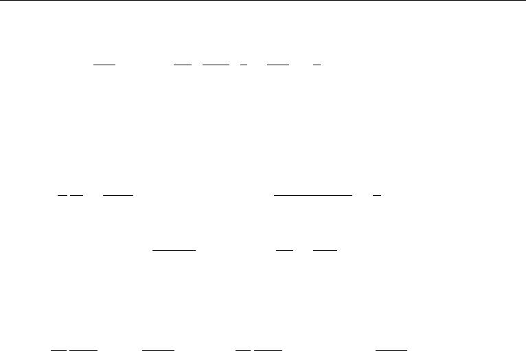
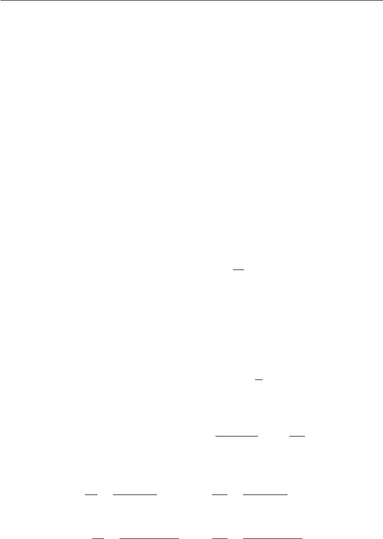
Figure 17.14 shows velocity profiles at intervals of ωt = 15
◦
, of the flow
resulting from a pressure gradient varying as cos(ωt) in a tube. As this is harmonic
motion, only half cycle is illustrated and for ωt > 180
◦
, the velocity profiles are of
the same form but opposite in sign. α is the Womersley number. The reversal of flow
starts in the laminae near the wall. As the Womersley number increases, the profiles
become flatter in the central region, there is a reduction in the amplitudes of the flow,
and the rate of reversal of flow increases close to the wall. At α = 6.67, the central
mass of the fluid is seen to reciprocate like a solid core.
806 Introduction to Biofluid Mechanics
Figure 17.14 Velocity profiles of a sinusoidally oscillating flow in a pipe. (Reproduced from McDonald,
D. A. (1974) Blood Flow in Arteries, The Williams & Wilkins Company, Baltimore).
Effect of Viscoelasticity of Tube Material
In general, the wall of a blood vessel must be treated as viscoelastic. This means
that the relations given in equations (17.104) and (17.105) must be replaced by
corresponding relations for a tube of viscoelastic material. In this problem, all the
stresses and strains in the problem are assumed to vary as e
i(kx−ωt)
, and we will
further assume that the effect of the strain rates on the stresses is small compared to
the effect of the strains. For the purely elastic case, only two real elastic constants
were needed. Morgan and Kiely (1954) have shown that by substituting suitable
complex quantities for the elastic modulus and the Poisson’s ratio the viscoelastic
behavior of the tube wall may be accommodated. They introduce,
E
∗
= E − iωE
, and, ˆν
∗
=ˆν − iωˆν
, (17.137)
where, E
and ˆν
are new constants. In equations (17.104) and (17.105), E
∗
and ˆν
∗
will replace E and ˆν, respectively. The formulation will otherwise remain the same.
An equation for k/ω will arise as before. The fact that E
∗
and ˆν
∗
are complex has
to be taken into account while evaluating the wave velocity and the damping factor.
Morgan and Kiely provide results appropriate for small and large α.
Morgan and Ferrante (1955) have extended the study by Morgan and Kiely
(1954) discussed above to the situation for small α values where there is Poiseuille
like flow in the thin, elastic walled tube. The flow oscillations are small and they are
superimposed on a large steady stream velocity. The steady flow modifies the wave
velocity. The wave velocity in the presence of a steady flow is the algebraic sum
3. Modelling of Flow in Blood Vessels 807
of the normal wave velocity and the steady flow velocity. Morgan and Ferrante
predict a decrease in the damping of a wave propagated in the direction of the
stream and an increase in the damping when propagated upstream. However, the
steady flow component in arteries is so small in comparison with the pulse wave
velocity that its role in damping is of little importance (see McDonald (1974)).
Womersley (1957a) has considered the situation where the flow oscillations are
large in amplitude compared to the mean stream velocity. This is similar to the
situation in an artery. He predicts that the presence of a steady stream velocity
would produce a small increase in the damping.
Next, we will study blood flow in branching tubes.
Blood Vessel Bifurcation: An Application of Poiseuille’s Formula and
Murray’s Law
Blood vessels bifurcate into smaller daughter vessels which in turn bifurcate to even
smaller ones. On the basis that the flow satisfies Poiseuille’s formula in the parent
and all the daughter vessels, and by invoking the principle of minimization of energy
dissipation in the flow, we can determine the optimal size of the vessels and the
geometry of bifurcation. We recall that Hagen-Poiseuille flow involves established
(fully developed) flow in a long tube. Here, for simplicity, we will assume that estab-
lished Poiseuille flow exists in all the vessels. This is obviously a drastic assumption
but the analysis will provide us with some useful insights.
Let the parent and daughter vessels be straight, circular in cross section, and lie
in a plane.
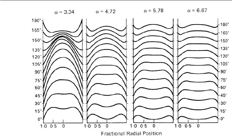
Consider a parent vessel AB of length L
0
of radius a
0
in which the flow rate is Q
which bifurcates into two daughter vessels BC and BD with lengths L
1
, and L
2
, radii
a
1
and a
2
, and flow rates Q
1
and Q
2
, respectively. The axes of vessels BC and BD
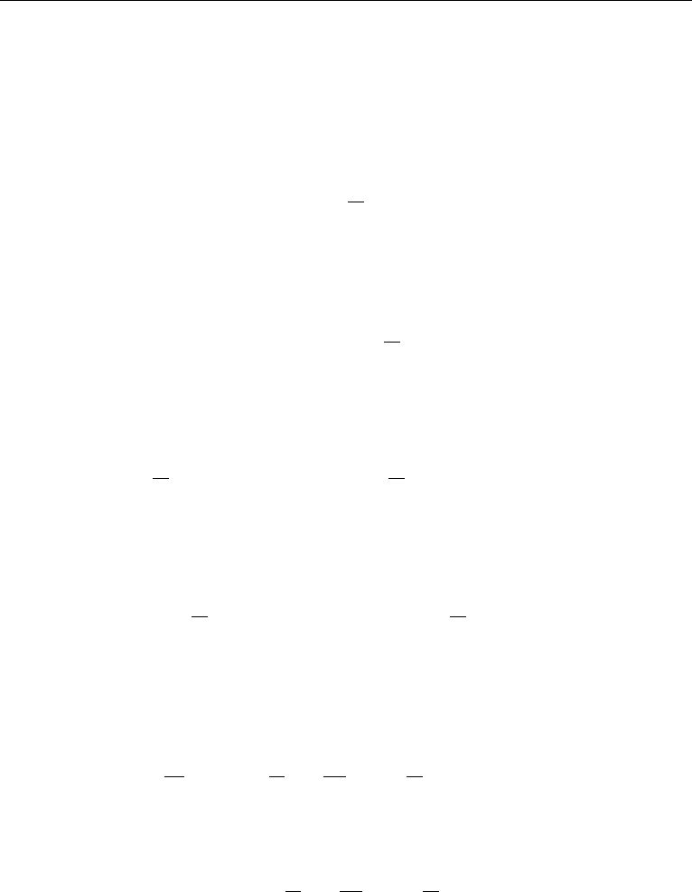
are inclined at angles θ and φ with respect to the axis of AB, as shown in Fig. (17.15).
Points A,C,D are fixed. The optimal sizes of the vessels and the optimal location of
B have to determined from the principle of minimization of energy dissipation.
Figure 17.15 Schematic of an arterial bifurcation.

808 Introduction to Biofluid Mechanics
The total rate of energy dissipation by flow rate Q in a blood vessel of length
of L and radius a is equal to sum of the rate at which work is done on the blood,
Qp, and the rate at which energy is used up by the blood vessel by metabolism,
Kπa
2
L, where K is a constant. For Hagen-Poiseuille flow, from equation (17.17),
Q =
πa
4
8µ
p
L
. Therefore,
Total energy dissipation =
8µL
πa
4
Q
2
+ Kπa
2
L =
ˆ
E
1
,(say). (17.138)
To obtain the optimal size of a vessel for transport, for a given length of vessel, we
need to minimize this quantity with respect to radius of the vessel. Thus,
∂
ˆ
E
1
∂a
=−
32µL
π
Q
2
a
−5
+ 2KπLa = 0. (17.139)
Solving for a,
a =
16µ
π
2
K
1/6
Q
1/3
. (17.140)
The equation (17.140) gives the optimal radius for the blood vessel indicating that
minimum energy dissipation occurs under this condition. The optimal relationship,
Q ∼ a
3
, is called Murray’s Law.
With equation (17.140), the minimum value for energy dissipation is
ˆ
E
1,min
=
3π
2
KLa
2
. (17.141)
Next, consider the flow with the branches. The minimum value for energy dissipation
with branches is
ˆ
E
2,min
=
3π
2
K
L
0
a
2
0
+ L
1
a
2
1
+ L
2
a
2
2
. (17.142)
Also,
a
0
=
16µ
π
2
K
1/6
Q
1/3
0
,a
1
=
16µ
π
2
K
1/6
Q
1/3
1
, and,a
2
=
16µ
π
2
K
1/6
Q
1/3
2
,
(17.143)
and, from mass conservation,
Q = Q
1
+ Q
2
→ a
3
0
= a
3
1
+ a
3
2
. (17.144)
The lengths L
0
,L
1
,L
2
depend on the location of point B. The optimum location of
the point B is determined by examining associated variational problems (see Fung
(1997)).
3. Modelling of Flow in Blood Vessels 809
Any small movement of B changes
ˆ
E
2,min
by δ
ˆ
E
2,min
, and,
δ
ˆ
E
2,min
=
3π
2
K
δL
0
a
2
0
+ δL
1
a
2
1
+ δL
2
a
2
2
(17.145)
The optimal location of B would be such as to make δ
ˆ
E
2,min
= 0 for arbitrary small
movement δL of point B. By making such displacements of B, one at a time, in the
direction of AB, in the direction of BC, and finally in the direction of DB, and setting
the value of the corresponding δ
ˆ
E
2,min
to zero, we develop a set of three conditions
governing optimization. These are:
cos θ =
a
4
0
+ a
4
1
− a
4
2
2a
2
0
a
2
1
, cos φ =
a
4
0
− a
4
1
+ a
4
2
2a
2
0
a
2
2
, cos(θ +φ) =
a
4
0
− a
4
1
− a
4
2
2a
2
1
a
2
2
.
(17.146)
Together with equation (17.144), equation set (17.146) may be solved for the optimum
angle θ as,
cos θ =
a
4
0
+ a
4
1
−
a
3
0
− a
3
1
4/3
2a
2
0
a
2
1
, (17.147)
and a similar equation for φ. Comparison of these optimization results with experi-
mental data are noted to be excellent (see Fung (1997)).
Reflection of Waves at Arterial Junctions: Inviscid Flow and Long Wave
Length Approximation
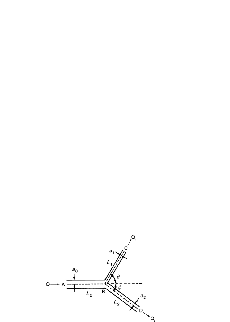
Arteries have branches. When a pressure or a velocity wave reaches a junction where
the parent artery 1 bifurcates into daughter tubes 2 and 3 as shown in the Figure 17.16,
the incident wave is partially reflected at the junction into the parent tube and partially
transmitted down the daughters. In the long wave length approximation, we may
neglect the flow at the junction. Let the longitudinal coordinate in each tube be x,
Figure 17.16 Schematic of an arterial bifurcation: Reflection.
810 Introduction to Biofluid Mechanics
with x = 0 at the bifurcation. the incident wave in the parent tube comes from
x =−∞.
Let p
I
be the oscillatory pressure associated with the incident wave, p
R
that asso-
ciated with the reflected wave, and p
T 1
and p
T 2
, those associated with the transmitted
waves. Let the pressure be a single valued and continuous function at the junction for
all time t. The continuity requirement ensures that there are no local accelerations.
Under these conditions, at the junction,
p
I
+ p
R
= p
T 1
= p
T 2
. (17.148)
Next, let Q
I
be the flow rate associated with the incident wave, Q
R
that associated with
the reflected wave, and Q
T 1
and Q
T 2
, those associated with the transmitted waves.
The flow rate is also taken to be single valued and continuous at the junction for all
time t. The continuity requirement ensures conservation of mass. At the junction,
Q
I
− Q
R
= Q
T 1
+ Q
T 2
. (17.149)
Let the undisturbed cross sectional areas of the tubes be A
1
, A
2
, and A
3
, and the
intrinsic wave speeds be c
1
, c
2
, c
3
, respectively. In general, for a fluid of density ρ
flowing under the influence of a wave with intrinsic wave speed c, through a tube of
cross sectional area A, the flow rate Q is related to the mean velocity u by,
Q = Au =±
A
ρc
p, (17.150)
where we have employed the relationship given in equation (17.68). The plus or the
minus sign applies depending on whether the wave is going in the positive x direction
or in the negative x direction. The quantity A/ρc is called the characteristic admittance
of tube and is denoted by Y , while, ρc/A, is called the characteristic impedance of
the tube and is denoted by Z. Admittance is seen to be the ratio of the oscillatory
flow to the oscillatory pressure when the wave goes in the direction of +x axis. With
these definitions,
Q = Au =±Yp =±
p
Z
. (17.151)
The equation (17.149) may be written in terms of admittances or impedances as:
Y
1
(p
I
− p
R
) =
3
j=2
Y
j
p
Tj
, or
(p
I
− p
R
)
Z
1
=
3
j=2
p
Tj
Z
j
. (17.152)
We can simultaneously solve equations (17.148) and (17.152) to produce,
p
R
p
I
=
Y
1
−
Y
j
Y
1
+
Y
j
= R, and
p
Tj
p
I
=
2Y
1
Y
1
+
Y
j
= T , (17.153)
or,
p
R
p
I
=
Z
−1
1
−
Z
−1
j
Z
−1
1
+
Z
−1
j
, and
p
Tj
p
I
=
2Z
−1
1
Z
−1
1
+
Z
−1
j
. (17.154)
3. Modelling of Flow in Blood Vessels 811
In equation (17.153), R and T are called the reflection and transmission coefficients,
respectively. From equation (17.153), the amplitudes of the reflected and transmitted
pressure waves are R and T times the amplitude of the incident pressure wave,
respectively. These relations can be written in more explicit manner as follows (see
Lighthill (1978)):
The contribution of the incident wave to the pressure in the parent tube is given
by,
p
I
= P
I
f
t −
x
c
1
, (17.155)
where, P
I
is an amplitude parameter, and f is a continuous, periodic function whose
maximum value is 1. The corresponding contribution to the flow rate is,
Q
I
= A
1
u = Y
1
P
I
f
t −
x
c
1
. (17.156)
The contributions to pressure from the reflected and transmitted waves to the parent
and daughter tubes, respectively, are:
p
R
= P
R
g
t +
x
c
1
, and,p
Tj
= P
Tj
h
j
t −
x
c
j
,(j= 2, 3). (17.157)
where P
R
and P
T
are amplitude parameters, and g and h are are continuous, periodic
functions. The corresponding contributions to the flow rates are:
Q
R
=−Y
1
P
R
g
t +
x
c
1
, and,Q
Tj
= Y
j
P
Tj
h
j
t −
x
c
j
,(j= 2, 3).
(17.158)
Therefore, the pressure perturbation in the parent tube is given by equation (17.155)
and (17.157) to be:
p
P
I
= f
t −
x
c
1
+
P
R
P
I
f
t +
x
c
1
, (17.159)
and the flow rate, from equations (17.156) and (17.158), is:
Q = Y
1
P
I
f
t −
x
c
1
−
P
R
P
I
f
t +
x
c
1
. (17.160)
The transmission of energy by the pressure waves is of interest. The rate of work
done by the wave motion through the cross section of the tube or equivalently, the
rate of transmission of energy by the wave is clearly, pAuor pQ, which is the same