Численные методы турбулентных несжимаемых течений (Том 4 Часть 2)

Подождите немного. Документ загружается.

14.3 Well-Posedness According to Hadamard 115

The basic ideas follows a standard approach in Functional Analysis and

can be concisely expressed as follows: Writing as above the NS equations in

pointwise form as R(ˆu) = 0 with ˆu = (u, p), we view R(·) as a residual van-

ishing pointwise for the solution ˆu. In this setting we seek a strong solution ˆu

which can be diﬀerentiated and thus satisﬁes the equation R(ˆu) = 0 pointwise

in space-time.

We now ﬁrst relax the requirements on ˆu, and deﬁne ˆu to be a weak solution

((R(ˆu), ˆv)) = 0,

for all test functions ˆv in a test space

V with norm k·k

consisting of suitably

pointwise diﬀerentiable functions, and R(ˆu) is assumed to belong to a space

dual to

V , and ((·, ·)) denotes a duality pairing. Eﬀectively this means that we

relax the regularity requirements on the solution ˆu and only ask the equation

R(ˆu) to be satisﬁed in some average sense depending on the test space

V . Typ-

ically, ((·, ·)) corresponds to a L

inner product in space-time and ((R(ˆu), ˆv))

is formally obtained by pointwise multiplication of R(ˆu) by the test function

ˆv and integration in space-time. It is the integration in space-time combined

with the regularity requirements put on the test functions that relaxes the

strong formulation R(ˆu) = 0 to the weak formulation ((R(ˆu), ˆv)) = 0 for all

ˆv ∈

V .

Next we relax further and deﬁne ˆu to be an -weak solution if

|((R(ˆu), ˆv))| ≤ kˆvk

∀ˆv ∈

V ,

where  is a (small) positive number. This means that for an -weak solution

ˆu, we require the residual R(ˆu) to be smaller than  in a weak norm which is

dual to the strong norm of

V . Choosing  = 0 would then bring us back to

Leray’s concept of an exact weak solution. Note that we here do not specify

precisely the space of functions where we seek the solution ˆu, but of course

we require that ˆu is such that ((R(ˆu), ˆv)) is well deﬁned for all ˆv ∈

V , or that

R(ˆu) belongs to the dual space of

V .

The ﬁnal step is now to choose an output quantity of interest and seek to

estimate the diﬀerence in output of two -weak solutions. This will lead us to

introduce a certain linearized problem and measure its stability properties by

a certain stability factor S. The diﬀerence in output of two -weak solutions

will then be estimated by 2S.

Before proceeding to present details of the new possible formulation of

the Prize Problem, we connect to the concept of well-posedness according to

Hadamard.

14.3 Well-Posedness According to Hadamard

The general question of uniqueness directly couples to a question about well-

posedness of a set of diﬀerential equations, as ﬁrst studied by the French math-

ematician Jacques Salomon Hadamard A set of partial diﬀerential equations

116 14 A $1 Million Prize Problem

(like the NS equations) is well-posed if small variations in data (like initial

data) result in small variations in the solution (at a later time). Hadamard

stated that only well-posed mathematical models could be meaningful: if very

small changes in data could cause large changes in the solution, it would clearly

be impossible to reach the basic requirement in science of reproducibility.

The question of well-posedness may alternatively be viewed as a question

of sensitivity to perturbations. A problem with very strong sensitivity to per-

turbations would not be well-posed in the Hadamard sense. Now Hadamard

proved the well-posedness of some basic partial diﬀerential equations like the

Poisson equation, but he did not state any result for the NS equations.

Of course, believing that solutions to the NS equations may be turbulent,

and observing the seemingly pointwise chaotic nature of turbulence, we could

not expect the NS equations to be well-posed in a pointwise sense: we would

expect to see a very strong pointwise sensitivity to small perturbations. But,

of course it would be most natural to ask if certain mean values may be less

sensitive, so that the NS equations would be well-posed in the sense of such

mean values. This is what we will do. The stability factor S may then be

viewed to measure the well-posedness of certain mean values in the sense of

Hadamard. Surprisingly maybe, this appears to be a new concept, which one

may describe as output uniqueness of approximate weak solutions as compared

to (non-existent) pointwise uniqueness of strong solutions.

14.4 -Weak Solutions

We now deﬁne the concept of -weak solutions of the NS equations (5.3) in

detail. We deﬁne for ˆv = (v, q) ∈

((R(ˆu), ˆv)) ≡ (( ˙u, v)) + (u(0), v(0)) + ((u ·∇u, v)) − ((∇ · v, p))

+ ((∇ · u, q)) + ((ν∇u, ∇v)) − (u

, v(0)) − ((f, v)),

(14.1)

where we choose

V = {ˆv = (v, q) ∈ H

(Q)

: v = 0 on Γ ×I}

and ((·, ·)) is the L

(Q)

inner product with m = 1, 3 (or a suitable duality

pairing) over the space-time domain Q = Ω ×I, and (·, ·) is the L

(Ω)

inner

product. Here H

(Q) denotes the Sobolev space of functions deﬁned on Q with

ﬁrst order derivatives in space-time in L

(Q), and H

(Q)

= H

(Q) ×H

(Q)

et cet. In order for all the terms in the deﬁnition of ((R(ˆu), ˆv)) to be deﬁned,

we thus ask (for example) that u ∈ L

(I; H

(Ω)

), (u·∇)u ∈ L

(I; H

−1

(Ω)

˙u ∈ L

(I; H

−1

(Ω)

), p ∈ L

(I; L

(Ω)), f ∈ L

(I; H

−1

(Ω)

), where H

(Ω)

is the usual Sobolev space of vector functions being zero on the boundary

Γ and square integrable together with their ﬁrst order derivatives over Ω,

with dual H

−1

(Ω). As usual, L

(I; X) with X a Hilbert space denotes the

14.4 -Weak Solutions 117

Hilbert space of functions v : I → X which are square integrable, with norm

kvk

(I;X)

= (

kv(t)k

)

1/2

We note that we could have chosen

V diﬀerently, asking for more or less

smoothness; e.g. we may demand more smoothness and ask

V to be a subset

of the Sobolev space H

(Q)

of vector functions with square integrable second

order derivatives. The choice of

V we made above ﬁts into the G2 formulation

to be given below.

We now deﬁne ˆu to be an -weak solution if

|((R(ˆu), ˆv))| ≤ kˆvk

∀ˆv ∈

V , (14.2)

where k·k

denotes the H

(Q)

-norm. We may here without loss of generality

put in requirements on some smoothness of ˆu, e.g. that ˆu ∈

V , or even the

more stringent requirement that R(ˆu) ∈ L

(Q)

, with R(ˆu) the residual of

(5.3). This is because we use a concept of approximate weak solution, which

allows us to smooth an approximate weak solution with minimal smoothness

requirements to get a smooth approximate weak solution. This reﬂects that

for any function v ∈ L

(Q), there is a smooth function v



(e.g. in H

(Q)),

such that kv − v



k ≤ , where k · k is the L

(Q)-norm. We also note that the

initial condition u(0) = u

is imposed approximately through the variational

formulation (14.1).

We now ﬁnally deﬁne



to be the set of -weak solutions (in

V ) for a

given  > 0. Equivalently, we may say that ˆu ∈

V is an -weak solution if

kR(ˆu)k

≤ ,

where k · k

is the dual norm of

V . This is a weak norm measuring mean

values of R(ˆu) with decreasing weight as the size of the mean value decreases.

Point values of R(ˆu) are thus measured very lightly. As indicated, we could

go to an even weaker solution concept, for example by replacing H

by H

We could also alternatively deﬁne



to be the set of functions ˆu such

that ((R(ˆu), ˆv)) = kˆvk

for all ˆv ∈

V , with = , but we prefer here the ﬁrst

deﬁnition with ≤ .

Formally, we would obtain the equation

((R(ˆu), ˆv)) = 0

by multiplying the NS equation by ˆv, that is, integrating in space-time the sum

of the momentum equation multiplied by v and the incompressibility equation

multiplied by q. Thus, a pointwise solution ˆu to the NS equations would be

an -weak solution for all  ≥ 0, while an -weak solution for  > 0 may be

viewed as an approximate weak solution, but not as an approximate pointwise

solution, because its pointwise residual may be large as well as kR(ˆu)k

(Q)

while kR(ˆu)k

is small.

Note that we may view an -weak solution ˆu to be a pointwise deﬁned

solution, like a ﬁnite element solution, for which the residual R(ˆu) is small in

the weak

-norm, but not in the L

(Q)-norm.

118 14 A $1 Million Prize Problem

14.5 Existence of -Weak Solutions by Regularization

There is a great variety of so called regularized NS equations for which it

is possible to prove existence of pointwise solutions using standard methods

of mathematical analysis. The regularization could be imposed by a higher-

order diﬀusion term like the biLaplacian with a small coeﬃcient acting on

the velocity, or replacing the velocity-independent Newtonian viscosity ν by

a viscosity ˆν depending on the norm of the velocity gradient with e.g.

ˆν = ν + h

|∇u|

where |∇u|

|∇u

, α ≥ 1 and h acts as a (small) scaling parameter.

For such regularized NS equations it is possible to prove the existence and

uniqueness of solutions (see e.g [81, 51]).

The question is then if such regularized solutions would be -weak solu-

tions, with an  tending to zero with the regularization? In general we would be

able to answer this question by yes, if we just use a suﬃciently weak solution

concept. The easiest case to analyze is regularization with the biLaplacian,

corresponding to introducing the additional viscous term ((κ∆u, ∆v)) in the

weak form of the NS equations, where κ > 0 is a small regularization param-

eter. We denote the corresponding regularized solution by ˆu

, which can be

proved to exist by standard methods. By a basic energy estimate, we would

have that ((κ∆u

, ∆u

)) ≤ C, where C would depend only on data. Com-

puting ((R(ˆu

), ˆv)) we would get by Cauchy’s inequality, assuming C = 1 for

simplicity,

|((R(ˆu

), ˆv))| = |((κ∆u

, ∆v))| ≤

√

κkˆvk

(I;H

(Ω)

)

so that ˆu

would be an

√

κ-weak solution with the norm of

V including the

(I; H

(Ω)

)-norm on the velocities.

Further, the original proof of Leray [79] produces a solution which is an

-weak solution for  = 0, if we impose on

V a slightly stronger norm on the

velocities than L

(I; H

(Ω)

), see [79, 81].

By introducing the notion of an -weak solution to the NS equations with

a suitable choice of norms on the test functions, it is thus possible to prove

existence of solutions using standard methods of mathematical analysis. Be-

low, we shall computationally construct -weak solutions using the G2 ﬁnite

element method (under a certain minor assumption). In general, for a com-

puted G2 solution

U, we can by evaluating the residual R(

U) determine the

corresponding .

To sum up, we may say that the question of existence of -weak solutions of

the NS equations is easy to settle, analytically or computationally. By relaxing

the requirements on the solution we have made the existence question easy to

answer positively. We now turn to the real issue.

14.6 Output Sensitivity and the Dual Problem 119

14.6 Output Sensitivity and the Dual Problem

Suppose now the quantity of interest, or output, related to a given velocity u

is a scalar quantity of the form

M(ˆu) = ((ˆu,

ψ)), (14.3)

where

ψ ∈ L

(Q) is a given weight function, which represents a mean-value

in space-time. In typical applications the output could be a drag or lift coeﬃ-

cient in a bluﬀ body problem. In this case the weight

ψ is a piecewise constant

in space-time. More generally,

ψ may be a piecewise smooth function corre-

sponding to a mean-value output.

We now seek to estimate the diﬀerence in output of two diﬀerent -weak

solutions ˆu = (u, p) and ˆw = (w, r). We thus seek to estimate a certain form

of output sensitivity of the space



of -weak solutions. To this end, we

introduce the following linearized dual problem of ﬁnding ˆϕ = (ϕ, ι) ∈

V such

that

a(ˆu, ˆw; ˆv, ˆϕ) = ((ˆv,

ψ)), ∀ˆv ∈

, (14.4)

where

= {ˆv ∈

V : v(·, 0) = 0}, and

a(ˆu, ˆw; ˆv, ˆϕ) ≡ (( ˙v, ϕ)) + ((u · ∇v, ϕ)) + ((v · ∇w, ϕ))

− ((∇ · ϕ, q)) + ((∇ · v, ι)) + ((ν∇v, ∇ϕ)),

with u and w acting as coeﬃcients, and

ψ is given data.

This is a linear convection-diﬀusion-reaction problem in variational form,

with u acting as the convection coeﬃcient and ∇w as the reaction coeﬃcient,

and the time variable runs “backwards” in time with initial value (ϕ(·,

t ) = 0)

given at ﬁnal time

t imposed by the variational formulation. The reaction

coeﬃcient ∇w may be large and highly ﬂuctuating, and the convection velocity

u may also be ﬂuctuating.

Choosing now ˆv = ˆu − ˆw in (14.4), we obtain

((ˆu,

ψ)) − (( ˆw,

ψ)) = a(ˆu, ˆw; ˆu − ˆw, ˆϕ) = ((R(ˆu), ˆϕ)) − ((R( ˆw), ˆϕ)), (14.5)

and thus we may estimate the diﬀerence in output as follows:

|M(ˆu) −M( ˆw)| ≤ 2kˆϕk

. (14.6)

By deﬁning the stability factor S(ˆu, ˆw;

ψ) = kˆϕk

, we can write

|M(ˆu) −M( ˆw)| ≤ 2S(ˆu, ˆw;

ψ), (14.7)

and by deﬁning



(

ψ) = sup

ˆu, ˆw∈



S(ˆu, ˆw;

ψ), (14.8)

we get

120 14 A $1 Million Prize Problem

|M(ˆu) −M( ˆw)| ≤ 2S



(

ψ), (14.9)

which expresses output uniqueness of



Clearly, S



(

ψ) is a decreasing function of  and we may expect S



(

ψ) to

tend to a limit S

(

ψ) as  tends to zero. For small , we thus expect to be able

to simplify (14.9) to

|M(ˆu) −M( ˆw)| ≤ 2S

(

ψ). (14.10)

Depending on

ψ, the stability factor S

(

ψ) may be small, medium, or

large, reﬂecting diﬀerent levels of output sensitivity, with S

(

ψ) increasing as

the mean value becomes more local. Normalizing, we may expect the output

M(ˆu) ∼ 1, and then one would need 2S

(

ψ) < 1 in order for two -weak

solutions to have a similar output.

Estimating S

(

ψ) in terms of the data

ψ, using a standard argument based

on multiplication by an integrating factor, would give a bound of the form

(

ψ) ≤ e

, where G a pointwise bound of |∇w|. In a turbulent ﬂow with

Re = 10

, we may have G ∼ 10

, and with

t = 10 we would have S

(

ψ) ≤

∼ e

10000

, which is an incredibly large number, larger than a googol= 10

100

It would be inconceivable to have  < 10

−100

and thus the output of an -weak

solution would not seem to be well deﬁned.

However, computing the dual solution corresponding to drag and lift co-

eﬃcients in turbulent ﬂow at Re = 10

, we ﬁnd values of S

(

ψ) which are

much smaller, in the range S

(

ψ) ≈ 10

, for which it is possible to choose  so

that 2S

(

ψ) < 1, with the corresponding outputs thus being well deﬁned (up

to a certain tolerance). We attribute the fact that ˆϕ and derivatives thereof

are not exponentially large, to cancellation eﬀects from the oscillating reac-

tion coeﬃcient ∇w. We shall study this aspect in model form more closely

below. However, the cancellation eﬀects seem to be impossible to account for

by analytical methods, because (i) knowledge of the underlying ﬂow velocity

u is necessary and (ii) the ﬂow velocity has a complexity defying analytical

description. The only way to get this knowledge is to compute the velocity,

and introducing computation, we may as well compute the dual solution to

get a computational hopefully reasonably accurate estimate of S

(

ψ), instead

of using a worst case estimate of no value at all. In practice, there is a lower

limit for , typically given by the maximal computational cost, and thus S

(

ψ)

eﬀectively determines the computability of diﬀerent outputs.

Note that we may view W



to be a set of possible (-weak) solutions sharing

a similar output up to the corresponding stability factor.

14.7 Reformulation of the Prize Problem

We now consider a couple of diﬀerent possible alternative formulations of

the Prize Problem. One could simply be our formulations (P) or (P1) from

Chapter 1. It seems that these problems could only be answered on a case by

14.7 Reformulation of the Prize Problem 121

case basis, so the Prize would have to be reformulated as a collection of say

1000 $1000 prizes, one for each case. In this book we cover a certain number

of these cases of key interest in applications.

We may compare with the following purely qualitative formulation which

could ﬁt into a tradition of “pure” mathematics dealing with exact solutions:

• (P2) What outputs of Leray’s weak solutions are unique?

In this book we present evidence indicating that (P2) is impossible to answer,

because of its purely qualitative nature. Instead we propose the quantitative

formulation (P1) involving approximate weak solutions. We could also formu-

late this problem as a problem of stability or sensitivity as follows:

• (P3) Determine output sensitivity of -weak solutions with  > 0, that is,

estimate the stability factor S



(

ψ) for  > 0 for diﬀerent ﬂows and diﬀerent

outputs (and diﬀerent norms for the test functions).

We have seen above that the diﬀerence in output given by a function

ψ of

two -weak solutions is at most 2S



(

ψ), which reﬂects the output sensitivity

in quantitative form. We may thus answer (P1) by answering (P3). One may

refer to (P3) as a question of weak uniqueness as a short for output sensitivity

of approximate weak solutions.

We remind the reader again that a Leray weak solution corresponds to a

-weak solution with  = 0. If S

(

ψ) < ∞, one could in purely qualitative form

argue that S



(

ψ) = 0 for  = 0, and output uniqueness of Leray solutions

would follow. However, as we said above, if S

(

ψ) is very large, this conclusion

could be misleading, because multiplication of 0 by ∞ is ill deﬁned. We thus

would conclude that (P2) may not be a mathematically sound formulation,

while the quantitative version (P3) should be.

In this book we thus only consider -weak solutions with  > 0. In fact

the concept of an 0-weak solution does not make much sense, since already a

weak solution is some kind of approximate solution in the pointwise sense. We

may then as well choose  > 0, and refrain from the possibly “pathological”

case  = 0!

In this book we address (P1), or (P3), using adaptive ﬁnite element meth-

ods with a posteriori error estimation. As indicated above the a posteriori

error estimate results from an error representation expressing the output er-

ror as a space-time integral of the residual of a computed solution multiplied

by weights which relate to derivatives of the solution of an associated dual

problem. The weights express sensitivity of a certain output with respect to

the residual of a computed solution, and their size determine the degree of

computability of a certain output: The larger the weights are, the smaller

the residual has to be and the more work is required. In general the weights

increase as the size of the mean value in the output decreases, indicating

increasing computational cost for more local quantities. The stability factor

(

ψ) is a certain space-time norm of the weights, and gives a scalar measure

of the output sensitivity.

122 14 A $1 Million Prize Problem

In the next chapter we present computational evidence in a bluﬀ body

problem that the drag coeﬃcient c

, which is a mean value in time of the drag

force, is computable to a reasonable tolerance at a reasonable computational

cost aﬀordable on a PC, while the value of the drag force at a speciﬁc point

in time appears to be uncomputable even at a very high computational cost.

14.8 The Standard Approach to Uniqueness

The standard approach to uniqueness of NS solutions goes as follows: Sup-

pose ˆu and ˆw are two classical pointwise solutions to the NS equations (5.3).

Subtracting the two versions of the NS equations, we obtain the following

equation for the diﬀerence ˆv = (v, q) = ˆu − ˆw:

˙v + (u · ∇)v + (v · ∇)w − ν∆v + ∇q = 0 in Ω × I,

∇ · v = 0 in Ω × I,

v = 0 on Γ ×I,

v(·, 0) = u

− w

in Ω,

(14.11)

Multiplying the momentum equation by v and integrating, we obtain for t ∈ I

kv(·, t)k

+ νk∇v(·, t)k

= −((v · ∇)w, v), (14.12)

where (·, ·) and k · k denote the scalar product and norm in L

(Ω)

for m =

1, 3, and we used the fact that since ∇ · u = 0, we have ((u · ∇v), v) = 0.

Estimating the right hand side by Gkvk

, where G as above is a pointwise

bound for ∇w, we obtain the following standard stability estimate:

kv(·,

t )k ≤ exp(G

t )ku

− w

We noted above that this estimate is void of content from any practical point

of view if G is large. Now, intense eﬀorts over many years have been made

to come up with alternative stability estimates involving only bounds on w

and not ∇w. This is possible using various Sobolev estimates as e.g in [81],

but will involve moving the derivative in ((v · ∇)w, v) instead to v and then

require using the ν-term in (14.12) in a stability estimate, and thus bring in an

exponential factor with exponent depending on negative powers of ν, which

again will be very large for high Reynolds numbers corresponding to small ν.

There is a classical type uniqueness result of this form stating uniqueness

if w ∈ L

(I; L

(Ω)) with

= 1 [81]. Since one can actually guarantee that

w ∈ L

(I; L

(Ω)) with

, it would seem that uniqueness would lie

around the corner, but again the presence of a very large exponential factor

means that this is only an illusion.

The net result seems to be that any conceivable stability estimate of clas-

sical type based on norm estimation of the crucial term ((v · ∇)w, v), which

does not use the oscillating character of the reaction coeﬃcient ∇w, would

necessarily involve very large stability factors and would thus be of no real

value, according to our point of view.

Weak Uniqueness by Computation

There’s no sense in being precise when you don’t even know what you’re

talking about. (John von Neumann)

Ces relations se d´eduisent d’ailleurs des ´equations de Navier–Stokes `a l’aide

d’int´egration par parties...j’ai pu d´emontrer le suivant: les relations en ques-

tion poss´edent toujours au moins une solution...Peut-ˆetre cette solution est-

elle trop peu r´eguli`ere pour poss´eder `a tout instant des d´eriv´ees secondes

born´ees; alors elle n’est pas, au sense propre du terme, une solution des

´equations de Navier–Stokes; je propose de dire qu’elle en constitute “une

solution turbulente” (Leray 1934).

15.1 Introduction

To compute approximations of a stability factor S



(

ψ) deﬁned by two -weak

solutions ˆu and ˆw approximately, we replace both ˆu and ˆw as coeﬃcients

in the dual problem by a computed -weak solution

U, such as a ﬁnite el-

ement solution, and then compute an approximate dual velocity ˆϕ

to get



(

ψ) ≈ S

(

ψ) ≡ kˆϕ

. We may then study S

(

ψ) as we reﬁne the

mesh size h, and we may extrapolate to h = ν to get an approximation of

(

ψ), assuming that h = ν would correspond to a small . If the extrapo-

lated value is not too large, then we would have evidence of output uniqueness,

and if the extrapolated value is very large, we would get indication of out-

put non-uniqueness. As a crude test of largeness it may be natural to use

(

ψ) >> ν

−1/2

If the output is a mean value, then kˆϕ

will typically grow slowly with

decreasing h. We may take this slow growth as evidence that it is possible to

replace both ˆu and ˆw by

U in the computation of the solution of the dual

problem: a near constancy indicates a desired robustness to (possibly large)

perturbations of the coeﬃcients ˆu and ˆw.

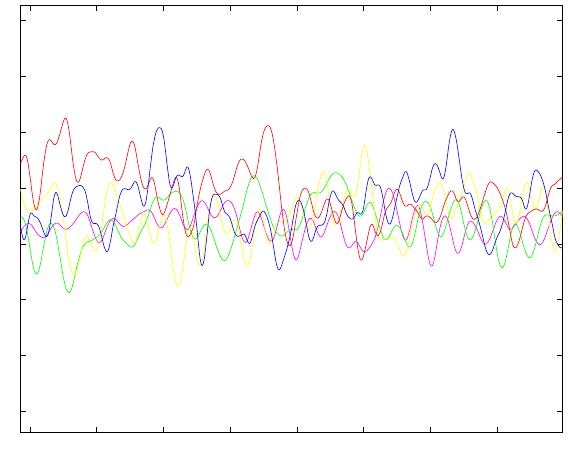
124 15 Weak Uniqueness by Computation

2 2.5 3 3.5 4 4.5 5 5.5

1.2

1.3

1.4

1.5

1.6

1.7

1.8

1.9

Fig. 15.1. Drag D(t) (normalized) for a surface mounted cube, as a function of

time, for 5 computational meshes.

15.2 Uniqueness of c

and c

The computational example is a bluﬀ body benchmark problem, which is

presented in more detail in Chapter 33. We compute the mean value in time

of drag and lift forces on a surface mounted cube in a rectangular channel, from

an incompressible ﬂuid governed by the NS equations (5.3), at Re = 40 000

based on the cube side length and the bulk inﬂow velocity. We compute the

mean values over a time interval of a length corresponding to 40 cube side

lengths, which we take as approximations of c

and c

deﬁned as (normalized)

mean values over very long time.

The incoming ﬂow is laminar time-independent with horse-shoe vortex up-

stream the cube and a laminar boundary layer on the front surface of the body,

which separates and develops a turbulent time-dependent wake attaching to

the rear of the body. The ﬂow is thus very complex with a combination of lam-

inar and turbulent features including boundary layers and a large turbulent

wake, see Figure 15.2.

The dual problem corresponding to c

has boundary data of unit size for

on the cube in the direction of the mean ﬂow, acting on the time interval

underlying the mean value, and zero boundary data elsewhere. A snapshot

of the dual solution corresponding to c

is shown in Figure 15.3, and in

Figure 15.4 we plot S

(

ψ) as a function of h

−1

for a range of adaptively