Chattaraj P.K. (Ed.) Quantum Trajectories

Подождите немного. Документ загружается.

364 Quantum Trajectories

In principle, the limit of any δ-function sequence [23] can be used in Equation 23.9, for

example the sinc-function sequence [24]. The Gaussian-based δ-function sequence,

δ(x) = lim

γ→∞

exp(−γx

), (23.10)

can be advantageous for many trajectory-based propagation methods (including the

AQPapproach) [3–7,9], because they are exact for Gaussian wavepackets and because

the initial wavefunction localized in coordinate space can be efﬁciently represented

with trajectories. Therefore, we approximate the eigensolution Equation 23.9 with

(x) =



2γ



1/4

exp(−γx

)



√

± ı



2γx



, λ =

√

8π

, (23.11)

choosing a large value of the width parameter γ which gives N (E) independent of γ.

Short-time analytical propagation in the parabolic approximation to the barrier can

be introduced to widen the highly localized initial wavefunction Equation 23.11 as

described in Ref. [15].

23.2.1 R

EAL-TIME VARIATIONAL APPROXIMATE QUANTUM POTENTIAL

The AQP method [9] is based on the quantum trajectory formulation [25, 26] of the

usual time-dependent Schrödinger equation (TDSE),



−



∇

+ V



ψ(x, t ) = ı

∂

∂t

ψ(x, t ). (23.12)

The wavefunction expressed in terms of the real amplitude A(x, t) and the real phase

S(x, t),

ψ(x, t ) = A(x, t )e

ıS(x,t)/

, (23.13)

is represented by an ensemble of trajectories characterized at time t by positions x

momenta p

and action functions S

. The trajectory momentum is the gradient of the

wavefunction phase,

p(x, t) =∇S(x, t). (23.14)

In the Lagrangian frame of reference,

∂

∂t

∇, (23.15)

Newton’s laws of motion for the quantum trajectories follow from the TDSE:

=−∇(V + U ), (23.16)

− (V +U ). (23.17)

Approximate Quantum Trajectory Dynamics in Imaginary and Real Time 365

The function U denotes the quantum potential,

U =−



∇

A(x, t )

, (23.18)

which vanishes in the classical limit  → 0 for nonzero wavefunction amplitudes.

The wavefunction density A

(x, t ) satisﬁes the continuity equation which, taking into

account evolution of the volume element δx

associated with each trajectory,

δx

= δx

exp





∇p

dτ



, (23.19)

results in conservation of the probability within δx

, i.e., of the trajectory “weight”

w(x

) = A

)δx

dw(x

)

= 0. (23.20)

Therefore, A(x, t ) can be reconstructed from trajectory positions and weights.

The concept of the trajectory weights is central to the approximate implementa-

tion of Equations 23.16 and 23.17 of Garashchuk and Rassolov [9, 27]. The AQP

(labeled

U) is determined variationally, thus conserving the energy of the trajectory

ensemble, from linearization of the nonclassical component, r(x, t ), of the momentum

operator:

r(x, t) =

∇A(x, t )

A(x, t )

. (23.21)

Minimization of (r −˜r)

, where ˜r is a linear function, has a solution in terms of the

moments of the trajectory distribution:

r(x, t) ≈˜r(x, t) =−

x −x

2(x



−x

)

. (23.22)

U and its gradient are determined analytically,

U =−





˜r

(x, t ) +∇˜r(x, t)



. (23.23)

The AQP method is exact for Gaussian wavepackets and describes wavepacket

bifurcation, moderate tunneling, and zero-point energy for times dependent on the

anharmonicity of V . It is numerically cheap and stable due to the “mean-ﬁeld”-like

procedure of determining AQP: with Equation 23.20 the expectation values in Equa-

tion 23.22 are computed as sums over trajectories labeled with index k,

Ω(x)



Ω(x)A

(x, t )dx =



Ω(x

)δx



Ω(x

(k)

. (23.24)

Using the mixed wavefunction representation, the correlation functions of Equa-

tion 23.7 can also be computed as single sums over trajectories, without ﬁnding

A(x, t ).

366 Quantum Trajectories

23.2.2 WAVEPACKET EVOLUTION AND COMPUTATION OF CORRELATION FUNCTIONS

IN THE

MIXED COORDINATE/POLAR REPRESENTATION

To propagate the ﬂux operator eigenfunctions Equation 23.11, we use the mixed

coordinate/polar wavefunction representation introduced in Ref. [16],

φ(x, t ) = ψ(x, t )χ(x, t), (23.25)

where ψ(x, 0) is a normalized Gaussian and χ(x, 0) is its polynomial prefactor. The

coordinate part, χ(x, t), is represented in theTaylor basis

f (x) ={1, x, ...}of size N

χ(x, t ) =

f (x) ·!a(t). (23.26)

The polar part, ψ(x, t), is an initially nodeless function solving the TDSE Equa-

tion 23.12. Substitution of Equations 23.25 and 23.26 into the TDSE for φ(x, t),

multiplication by ψ

∗

(x, t )

f (x) and integration over x gives the matrix equation for

d !a/dt,

ı

f ⊗

f 

d !a



∇

f ⊗∇

f 

− ı

p

f ⊗∇

f 



!a. (23.27)

All integrals are evaluated according to Equation 23.24. For example, the matrix

elements of the last term of Equation 23.27 are

p

f ⊗∇

f 



(k)

)∇f

(k)

The polar part ψ(x, t ) is described in terms of quantum trajectories, initiated

with zero initial momenta at positions sampling the Gaussian part of φ

(x) given

by Equation 23.11, propagated in the presence of AQP. The functions χ

(x,0) =

(0) ± a

(0)x are the polynomial prefactors of φ

(x). Restricting χ

to a linear

form, for symmetric V the coefﬁcients are:

(t) = a

(0), a

(t) = a

(0) exp



−



px

+ ı/2

mx



dτ



. (23.28)

The mixed representation reduces the propagation error and cost, because it allows

for stable trajectory dynamics of the nodeless (at least for short time) ψ(x, t) and it

simpliﬁes calculations of the correlation functions, C

, in Equation 23.7. C

can be

expressed via the trajectory weights if the evolution operator is equally partitioned

between bra and ket,

(2t) =



(k)

2ıS

(k)



(t) + a

(t)x

(k)



(t) ∓ a

(t)x

(k)



. (23.29)

23.2.3 N

UMERICAL ILLUSTRATION

Here the wavepacket formulation of Equations 23.7, 23.8, and 23.11 is used to com-

pute the reaction probability, N (E), for a one-dimensional model of the H

transition

state—for the Eckart barrier scaled to have m = 1,

Approximate Quantum Trajectory Dynamics in Imaginary and Real Time 367

V = V

cosh

−2

αx. (23.30)

In scaled units the barrier height is V

= 16 and α = 1.3624 a

−1

The purpose was to assess the accuracy of the AQP description of the tunnel-

ing regime. The implementation was not optimized. The trajectory positions were

distributed uniformly. For linear χ(x, t), the only quantities needed to determine the

quantum force and the polynomial coefﬁcient a

in Equation 23.28 are x

and px,

which could be computed with relative errors below 2 ×10

−5

with 1000 trajectories.

We needed many more trajectories (10

) to obtain low-tunneling probabilities with

uniform sampling. The numerical cost scales linearly with the number of trajectories.

In principle, the AQP parameters and coefﬁcients !a can be simply stored from a cal-

culation with a few thousand trajectories and used to propagate a larger number of

independent trajectories, possibly, with more effective trajectory sampling.

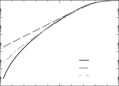
The cumulative reaction probability, N(E), obtained for γ = 1000 a

−2

is shown

in Figure 23.1. The trajectories were propagated up to t = 1.5, which, due to the

doubling of time in Equation 23.29, would be sufﬁcient to resolve probabilities above

−9

in a conventional QM wavepacket calculation. For energies below V

the AQP

probabilities above 10

−5

were quite accurate. The AQP probabilities below this value

were too high. Nevertheless, there was a noticeable improvement over the parabolic

barrier approximation: for E = 0.52, the lowest energy resolved, the parabolic barrier

dynamics overestimated N (E)by2×10

, while the AQP probability was 200 times

smaller than that. As argued in Ref. [9], out of the two approximations made—the

linear quantum force and the linear form of χ(x, t)—the former is the main source

of error.

10020

Energy

1e-10

1e-08

1e-06

0.0001

0.01

N(E)

Analytical

Parabolic

AQP

FIGURE 23.1 The cumulative reaction probability, N(E), for the Eckart barrier obtained

from propagation of the ﬂux eigenvectors using the AQP trajectory dynamics and mixed wave-

function representation. A comparison is made with the analytical QM probability and with

the probability derived from the analytical wavefunctions evolving in the parabolic potential

in Equations 23.7 and 23.8.

368 Quantum Trajectories

23.3 TRAJECTORY DYNAMICS IN IMAGINARY TIME WITH

THE MOMENTUM-DEPENDENT QUANTUM POTENTIAL

Direct computation of the reaction rate constants according to Equations 23.3 and 23.4

requires Boltzmann evolution of wavefunctions, equivalent to propagation in imagi-

nary time. Another type of problem solvable in imaginary time is the determination

of low-lying energy levels and eigenfunctions [28], in particular of the energy levels

in high-dimensional systems with Monte Carlo methods [29–31]. The approach is

based on the simple fact that in imaginary time,

H ψ(x, τ) =−

∂ψ(x, τ)

∂τ

, τ > 0 (23.31)

the higher energy components of a wavefunction ψ(x, τ) decay faster than the lower

energy components: a wavefunction expressed in terms of the eigenstates {ψ

} of

> 0),

H ψ

(x) = E

(x), ψ(x, τ) =



−E

(x), (23.32)

decays to the lowest energy state of the same symmetry. Some recent examples are

calculations performed for malonaldehyde [32] and for CH

[33].

Substitution of the time variable, t →−ıτ (τ > 0), transforms the real-time

TDSE Equation 23.12 into the diffusion Equation 23.31. In semiclassical treatments

of Equation 23.31 [34, 35] transformation of p →−ıp and S →−ıS, led to the

classical equations of motion of trajectories in the “inverted” potential (the nega-

tive of the original V ). The same transformation of Equations 23.16, however, leads

to singular dynamics of a Gaussian wavefunction [36]. Such behavior is related to

the nonunique representation of a real wavefunction in terms of the amplitude and

“phase,” as Equation 23.13 becomes

ψ(x, τ) = A(x, τ)e

−S(x,τ)/

and re-partitioning of the wavefunction between A and S to avoid singularities was

successfully employed.

For a real positive wavefunction we use an unambiguous exponential form,

ψ(x, τ) = e

−S(x,τ)/

. (23.33)

The wavefunction Equation 23.33 is the same as in the Zero Velocity Complex Action

method of Ref. [37] implemented in imaginary time on a ﬁxed grid.

23.3.1 E

QUATIONS OF MOTION

Substitution of the wavefunction Equation 23.33 into Equation 23.31 and division by

ψ(x, τ) gives

∂S(x, τ)

∂τ

=−

(

∇S(x, τ)

)

+ V +



∇

S(x, τ). (23.34)

Approximate Quantum Trajectory Dynamics in Imaginary and Real Time 369

Using τ as a time variable and deﬁning the trajectory momentum by Equation 23.14

in the Lagrangian frame of reference Equation 23.15, Equation 23.34 leads to the

following equations of motion,

dτ

=∇(V + U ). (23.35)

Compared to the real-time equations 23.16 and 23.18, in imaginary time we have the

“inverted” potential and the MDQP,

U(x, τ) =



∇

S =

∇p

. (23.36)

Note that imaginary-time U (x, τ) is proportional to /m and, thus, vanishes in the

classical limit as its real-time counterpart Equation 23.18. In many dimensions Equa-

tion 23.36 generalizes to U (!x, τ) = 

∇·

∇S/(2m). Evolution of the imaginary-time

action function is

dτ

+ V +U , (23.37)

and the energy of a trajectory is

ε =

∂S

∂τ

=−

+ V +U . (23.38)

Remarkably, for the wavefunction Equation 23.33 evolution of the volume ele-

ment δx

given by Equation 23.19 cancels the contribution of MDQP to the average

quantities,

Ω=



∞

−∞

Ω(x)e

−2S(x)/

dx =



Ω(x

(k)

−2

/

δx

(k)

. (23.39)

S indicates the “classical” action function computed along the quantum trajectory,





+ V (x

)



dt. (23.40)

For a Gaussian wavefunction evolving in a quadratic potential, S(x, τ) is a quadratic

function of x, p(x, τ) is linear in x, U is a time-dependent constant and the quan-

tum force, ∇U , is zero. Therefore, average x-orp-dependent quantities of classical

(U = 0) and QM evolutions are the same. This quantum/classical similarity was one

of the motivations behind the real-time Bohmian mechanics with Complex Action

(BOMCA) in complex space [38].

23.3.2 A

PPROXIMATE IMPLEMENTATION AND EXCITED STATES

To implement Equations 23.35 and 23.37 one has to know derivatives of p determining

U and ∇U . Since our goal is a cheap approximate methodology, we ﬁnd derivatives

from the least squares ﬁt [39] to p(x, τ) weighted by ψ

(x, τ). Representing p(x, τ)

370 Quantum Trajectories

in a small basis

f (x) of size N

, p(x, τ) ≈

f (x) ·

b(τ), the optimal coefﬁcients

minimizing (p −

f ·

 are

b = M

−1

P . (23.41)

M is a time-dependent symmetric matrix of the basis function overlaps,

=f

=



(k)

) exp(−2

(k)

)δx

(k)

. (23.42)

The vector

P includes the trajectory momenta averaged with the basis functions,

=pf

=



(k)

) exp(−2

(k)

)δx

(k)

. (23.43)

Placing the minimum of V at x = 0 we use the Taylor basis,

f (x) = (1, x, x

, ...)

, (23.44)

to determine MDQP and to evolve wavefunctions with nodes in the mixed coordinate

space/trajectory representation analogous to Equation 23.25.

The nodeless ψ(x, τ) solving Equation 23.31 evolves in imaginary time into the

ground state wavefunction according to Equation 23.32. For χ(x, τ) represented in a

basis

f (x) of size N

χ(x, τ) =

f (x) ·!c(τ), (23.45)

the time-dependent coefﬁcients !c are obtained from Equation 23.31 proceeding as in

Section 23.2,

d !c

dτ

=−



−1

D!c. (23.46)

D is the matrix of the basis function derivatives,

=∇f

|∇f

=



∇f

(k)

)∇f

(k)

) exp(−2

(k)

)δx

(k)

. (23.47)

To ﬁnd the ground state of a system we start with a Gaussian ψ(x, 0), since its

evolution is exact in a quadratic potential for the smallest meaningful basis, N

= 2.

Although a linear approximation to p(x, τ) gives zero quantum force, which does not

affect the positions of the trajectories, MDQPis still required to deﬁne the total energy.

To obtain N

eigenstates we evolve N

mixed representation functions φ

= χ

(n = 1, ..., N

). The functions χ

are represented in the Taylor basis Equation 23.44,

and their coefﬁcients are written as a matrix C = (!c

, !c

, ..., !c

). The number of

states, N

, is no larger than the basis size, N

. The initial functions χ

will have the

correct number of nodes, if the initial values C

are chosen for φ

(x, 0) to be, for

example, the eigenfunctions of a harmonic oscillator.At each time step wavefunctions

of the lower energy are projected out:

new

= χ

−



k,k<j

χ

|χ

χ

, (23.48)

Approximate Quantum Trajectory Dynamics in Imaginary and Real Time 371

which in terms of C and the overlap matrix Equation 23.42 is

new

= C

−



k,k<j

χ

|χ

C

, χ

|χ

=(C

MC)

. (23.49)

Both the determination of MDQP and the evolution of C require inversion of the

overlap matrix M. For N

= N

the calculation of the excited states requires little

effort in addition to the quantum trajectory propagation. The outlined approach is

approximate and is expected to work for a few low-energy eigenstates where the

modest basis size is sufﬁciently accurate.

23.3.3 C

ALCULATION OF THE ENERGY LEVELS

The approximate MDQP approach is illustrated for anharmonic systems, which

proved to be challenging for real-time exact and approximate quantum trajectory

dynamics [40–42]. The difﬁculty is the inherent instability of the real-time Bohmian

trajectories describing stationary eigenstates: such trajectories should not move, there-

fore classical and quantum forces have to cancel each other exactly. Otherwise, small

displacements of the trajectory positions lead to rapid “decoherence” of the trajecto-

ries and, consequently, to the loss of quantum effects. In contrast, the imaginary-time

trajectories are not stationary—their dynamics reﬂects the decay of the wavefunction.

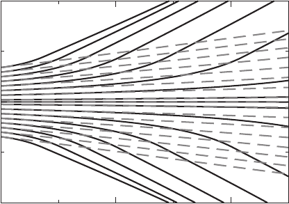
For the harmonic oscillator, the imaginary-time trajectories “roll off” a parabolic bar-

rier, which is the inverted well centered at x = 0, as shown on Figure 23.2. The same

is qualitatively true for anharmonic single-well potentials in one dimension.

0 0.2 0.4

Time

–10

Position

FIGURE 23.2 Imaginary-time quantum trajectories for the quadratic (dash) and quartic (solid

line) oscillators. The quantum potential is found approximately using N

= 4 for the latter

potential.

372 Quantum Trajectories

TABLE 23.1

The Energy Levels (n = 0, ..., 3) for the Anharmonic Well of Equation 23.50

Obtained from the Imaginary-Time QuantumTrajectory Dynamics.The Bottom

Line Contains the Exact QM Values from the Diagonalization of the Hamilto-

nian Matrix. In the HarmonicApproximation to the Potential, the Energy Levels

are E

quad

= n + 1/2

2 4 0.76007 2.3139 4.5298 7.1670

4 4 0.80358 2.7371 5.2856 8.2111

6 6 0.80375 2.7379 5.1829 7.9435

QM 0.80377 2.7379 5.1719 7.9424

For illustration we consider a particle of mass m = 1 a.u. in a well with quartic

anharmonicity [36],

V = x

+ x

/2. (23.50)

The parameter γ = 1a

−2

speciﬁes a Gaussian initial wavefunction,

ψ(x,0)=



2γ



1/4

−γx

, (23.51)

evolved up to τ = 1.0 a.u. using 500 trajectories. The trajectories corresponding to

V of Equation 23.50 and its quadratic part, V

quad

= x

/2, are shown on Figure 23.2.

Four basis functions, N

= 4, were used to deﬁne the MDQP for the full V . The

trajectories spread out faster in the anharmonic case, but the overall behavior is

similar to the dynamics in V

quad

Four lowest energy levels and wavefunctions were computed using four and six

functions to represent χ

. The initial values of C were taken as for the excited states of

the harmonic oscillator of frequency w = 2γ. The ground state energy of V exceeds

that of V

quad

by 60%. The linear ﬁtting (N

= 2) of the momentum, exact for the

harmonic oscillator, recovers 86% of the difference. Increasing N

gives energies

within four signiﬁcant ﬁgures of the exact QM calculation for nearly all levels as

summarized in Table 23.1.

The quantum trajectory results were essentially the same for γ = 2 and 0.5 a

−2

In general, the decay time and convergence to the ground state will depend on the

closeness of the initial wavefunction, ψ(x, 0), to the ground state and on the energy

levels. To obtain the highest energy eigenstate, n = 3, the projection procedure of

Equation 23.48 necessitated time steps as small as dτ = 10

−4

. This eigenstate is the

fastest to decay and, if the lower energy components are not removed from φ

(x, τ),

which is a mixture of eigenstates, very frequently, then this wavefunction can decay

to a lower energy eigenfunction.

Approximate Quantum Trajectory Dynamics in Imaginary and Real Time 373

TABLE 23.2

The Energy Levels for the Double Well for n = 0, ..., 3, Obtained with Approx-

imate MDQP, N

= N

= 6, and by the Diagonalization of the Hamiltonian

Matrix. The Initial Width Parameter is a = 0.75. The Normalized Energies of

are Computed at Time τ Listed in the Second Column

m [a.u.] τ [a.u.] E

1 2.0 0.397 1.122 2.395 3.842

QM 0.397 1.122 2.378 3.841

20 8.0 0.133 0.152 0.345 0.473

10.0 0.131 0.152 0.348 0.479

QM 0.133 0.152 0.332 0.465

The double well of Ref. [43], considered for m = 1 and m = 20,

V = (x

− 1)

/4, (23.52)

presents a more challenging application. As m is increased the ground state function

changes from a single peak to a double peak. The trajectory dynamics is more compli-

cated, because unlike purely divergent trajectories of single wells, in the double well

some trajectories stay in the barrier region. For m = 20, approximation of p(x, τ)

within a small basis did not give fully converged eigenfunctions. Using larger bases,

in principle, should give converged eigenvalues, but this was not pursued as it seemed

impractical.

Table 23.2 shows the four lowest energy levels computed with N

= N

= 6.

The initial width parameter is γ = 0.75 a

−2

for all calculations. The agreement of

the wavefunction energies with the exact QM energy levels is fairly good, though the

energies of φ

for m = 20 weakly depend on τ after initial decay. The accuracy of the

lower energy levels, which is better than 1.5%, resolves the E

−E

energy splitting

of 0.02 a.u.; the accuracy for n = 2 and 3 is 5 and 3%, respectively. The accuracy for

the m = 1 system is better than 1% for all levels. The ground state wavefunctions for

m = 1 and m = 20 are shown in Figure 23.3. Note that the double peak for m = 20

has evolved from the Gaussian function (without the polynomial prefactors).

23.4 COMPUTATION OF REACTION RATES FROM

THE IMAGINARY AND REAL-TIME QUANTUM

TRAJECTORY DYNAMICS

Now we are ready to compute the reaction rate constants using Equation 23.4 within

the approximate quantum trajectory dynamics in real and imaginary time and the

mixed wavefunction representation [44]. Boltzmann evolution of the singular ﬂux

operator eigenvectors composed of all energy components—the inﬁnite temperature

situation—can be viewed as “cooling.” Due to rapid decay of the high-energy com-

ponents the wavefunctions become nonsingular for any ﬁnite temperature. In fact, we