Chattaraj P.K. (Ed.) Quantum Trajectories

Подождите немного. Документ загружается.

344 Quantum Trajectories

4. D. Bohm, B. J. Hiley, and P. N. Kaloyerou, Phys. Rep. 144 (1987) 321.

5. D. Bohm and B. J. Hiley, The Undivided Universe, Routledge, London, 1993.

6. P. R. Holland, The Quantum Theory of Motion, Cambridge University Press, New York,

1993.

7. R. E. Wyatt, Quantum Dynamics with Trajectories: Introduction to Quantum Hydrody-

namics, Springer, New York, 2005.

8. C. Lopreore and R. E. Wyatt, Phys. Rev. Lett. 82 (1999) 5190.

9. R. E. Wyatt and E. R. Bittner, J. Chem. Phys. 113 (2000) 8898.

10. K. H. Hughes and R. E. Wyatt, Chem. Phys. Lett. 366 (2002) 336.

11. B. K. Kendrick, J. Chem. Phys. 119 (2003) 5805.

12. B. K. Kendrick, J. Molec. Struct.: THEOCHEM 943 (2010) 158–167.

13. J. Von Neumann and R. D. Richtmyer, J. Appl. Phys. 21 (1950) 232.

14. D. K. Pauler and B. K. Kendrick, J. Chem. Phys. 120 (2004) 603.

15. S. W. Derrickson, E. R. Bittner, and B. K. Kendrick, J. Chem. Phys. 123 (2005) 54107-1-9.

16. B. K. Kendrick, J. Chem. Phys. 121 (2004) 2471.

17. V. A. Rassolov and S. Garashchuk, J. Chem. Phys. 120 (2004) 6815.

18. S. Garashchuk, J. Phys. Chem. A 113 (2009) 4451.

19. C. J. Trahan, K. Hughes, and R. E. Wyatt, J. Chem. Phys. 118 (2003) 9911.

Bohmian Grids and the

Numerics of Schrödinger

Evolutions

D.-A. Deckert, D. Dürr, and P. Pickl

CONTENTS

22.1 Introduction.................................................................................................345

22.2 Problems of the Numerical Implementation...............................................349

22.3 Fitting Algorithms: What They Can Do and What They Can’t ..................352

22.4 A Numerical Example in MATLAB



........................................................355

Bibliography ..........................................................................................................359

22.1 INTRODUCTION

Bohmian mechanics [1, 2] is a mechanical theory about the motion of particles. In

contrast to quantum mechanics, Bohmian mechanics is a complete physical theory

which leaves no interpretational freedom; in particular, it is free of paradoxes like

Schrödinger’s cat. This completeness is achieved by introducing a deﬁnite conﬁgu-

ration of particles for all times which is governed by the Bohmian velocity law. The

predictions of Bohmian mechanics agree with those of quantum mechanics when-

ever the latter are unambiguous. Besides that, it turns out that in some situations

the Bohmian velocity law is a convenient tool for the numerical integration of the

Schrödinger equation. There is a lot of literature which explains the physical side

of Bohmian mechanics, see e.g. Ref. [2]. The role of this chapter is to explain the

advantages in using Bohmian mechanics for numerics.

Let us discuss the Bohmian equations of motion in units of mass m =  = 1. First,

one has the Schrödinger equation

dψ

(x)



−

∇

+ V (x)



(x) . (22.1)

Here x = (x

, ...,x

) denotes the conﬁguration in conﬁguration space R

. Fur-

thermore, we use the notation ∇

= (∇

, ...,∇

) where ∇

is the gradient with

respect to x

∈ R

Let ψ

be a solution of the N -particle Schrödinger equation with initial condi-

tion ψ

t=0

(x) = ψ

(x). Given the initial positions q

, ...,q

of the particles, the

Bohmian velocity law then determines the positions q

(t), ...,q

(t) of the particles

345

346 Quantum Trajectories

at any time t. In this way Bohmian mechanics describes for given ψ

and any given

initial conﬁguration q(0) := (q

)

1≤k≤N

the motion of the conﬁguration space trajec-

tory q(t) := (q

(t))

1≤k≤N

. Note that one such conﬁguration space trajectory describes

the motion of all N particles.

The trajectories of the N particles q

, ψ

;t) ∈ R

,1≤ k ≤ N , are solutions

of the Bohmian velocity law

(t)

= Im



∗

∇

∗

, ...,q

)



(22.2)

with q

(t = 0) = q

as initial conditions and ψ

∗

denoting the complex conjugate

of ψ, so that ψ

∗

ψ =|ψ|

. Interpreting ψ

∗

ψ as an inner product, the generalization

to spin wavefunctions is straightforward [2]. Using conﬁguration space language the

Bohmian trajectory of an N particle system is an integral curve q(t) ∈ R

of the

following velocity ﬁeld on conﬁguration space

(q, t) = Im



(ψ

∗

∇

)(q)

(ψ

∗

)(q)



, (22.3)

i.e.,

dq(t)

= v

(q, t). (22.4)

Statistical Bohmian Mechanics. Like in quantum mechanics the exact initial con-

ﬁguration q

of the N particles is unknown. One usually starts with a probability dis-

tribution for the initial conﬁguration given by the density |ψ

(Bohmian mechanics

explains why, see Ref. [2, 3]).

Therefore, in Bohmian mechanics one has to consider an ensemble of many con-

ﬁguration space trajectories which is initially |ψ

-distributed. Each of these conﬁg-

uration space trajectories describes a different possible physical time evolution of all

the N particles and must not be confused with different one-particle trajectories.

Under general conditions one has global existence and uniqueness of Bohmian

conﬁguration space trajectories, i.e., the integral curves do not run into nodes of the

wavefunctions and they cannot cross [4]. The uniqueness, i.e., non-crossing property,

is due to the fact that the Bohmian law is given by a velocity vector ﬁeld: at each

conﬁguration point there is a unique vector, prescribing the velocity of the conﬁg-

uration in that point. To avoid misunderstandings it is important to emphasize that

the non-crossing of Bohmian conﬁguration space trajectories has nothing to do with

possible crossings of particle paths. The crossing of particle paths is in fact allowed

in Bohmian mechanics. For example the situation where two particle paths cross at

time t

is described by just one Bohmian trajectory: at time t

the position of both

particles is equal, let’s say x

, i.e q(t

) = (x

, x

To analyze Bohmian mechanics statistically we must introduce an ensemble den-

sity ρ(q, t). Such a density fulﬁlls the continuity equation, which for the Bohmian

ﬂow reads

Bohmian Grids and the Numerics of Schrödinger Evolutions 347

∂ρ(x, t)

∂t

+∇



ρ(x, t )v

(x, t )



= 0.

The empirical import of Bohmian mechanics arises now from equivariance of the |ψ|

measure: one readily sees that by virtue of (Equation 22.3) the continuity equation

is identically fulﬁlled by the density ρ(x, t) =|ψ(x, t)|

, known as the quantum ﬂux

equation,

∂|ψ(x, t)|

∂t

+∇



|ψ(x, t )|

(x, t )



= 0.

In contrast to Hamiltonian statistical mechanics where typical trajectories are

described by stationary measures (like microcanonical or canoncial distributions)

in Bohmian mechanics the typical trajectories are described by the equivariant mea-

sure ρ(x, t) =|ψ(x, t)|

. In other words the notion of equivariance replaces the notion

of stationarity. This means that if one looks at an ensemble of Bohmian trajectories

such that the respective initial conﬁgurations q(0) = (q

, ...,q

) are distributed

according to ρ

=|ψ

, ...,x

at time t = 0, then for any time t the conﬁg-

urations q(t) = (q

, ψ

;t), ...,q

, ψ

;t)) are distributed according to ρ

|ψ

, ...,x

. Because of this, Bohmian mechanics agrees with all predictions

made by orthodox quantum mechanics whenever the latter are unambiguous [3,5].

Hydrodynamic Formulation of Bohmian Mechanics. In this section we recast the

Bohmian equations of motion in a form which is suitable for numerical analysis.

We ﬁrst write ψ in the Euler form

ψ(x, t ) = R(x, t )e

iS(x,t)

where R and S are real-valued functions. Equation 22.3 together with Equation 22.1

separated into their real and complex parts gives the following set of differential

equations (which are very much analogous to the Hamilton–Jacobi equation of

Hamiltonian mechanics)

=∇

S(q, t)

∂R(x, t)

∂t

=−

∇

(R(x, t)∇

S(x, t))

∂S(x, t)

∂t

=−

(

∇

S(x, t)

)

− V (r) +

∇

R(x, t )

We now introduce the functions R(t), S(t) deﬁned by replacing the conﬁguration point

x by the conﬁguration space trajectory q(t):

R(t) = R(q(t), t) S(t) = S(q(t), t).

Taking the derivatives with respect to time, for example,

dR(q(t), t)

∂R(q(t), t)

∂t

∂R(x, t)

∂x

x=q(t )

348 Quantum Trajectories

yields, using the notation q = q(t),

=∇

S(q, t) (22.5)

∂R(q, t )

∂t

=−

R(q, t)∇

S(q, t) (22.6)

∂S(q, t)

∂t





− V (q) +

∇

R(q, t)

. (22.7)

Numerical Integration. To solve a differential equation like the Schrödinger equa-

tion numerically one has to ﬁrst discretize the problem. Instead of the full function

ψ(x, t ) where x varies in conﬁguration space R

one considers ψ(x

, t

) where

, ...,x

and t

, ...,t

are discrete “grid” points in conﬁguration space and on the

time axis.

When choosing the grid one has to take care of the following two things:

• The values ψ(x

, t

) deﬁne an approximation

ψ for ψ. For example one could

think of

ψ(x, t ) = ψ(x

, t

) where for x

one chooses the grid point closest to

x and t

closest to t (as explained later one usually employs a ﬁtting algorithm

to compute the numerical approximation

ψ from the discrete data points

(ψ(x

, t

)

1≤k≤n,1≤l≤m

). To reproduce from this discretization the physically

relevant features of the full wavefunction one has to take care that the relevant

regions in conﬁguration space are well covered by the grid points.

The sense of approximation needed in physics is the L

-distance, i.e., in

the above example





ψ(x, t ) − ψ(x, t)|



1/2

. (22.8)

• Of course the choice of grid points also inﬂuences the propagation of errors,

as for example, the accuracy in computing derivatives depends on the grid.

In the usual approaches the grid points are ﬁxed once and stay ﬁxed for all times.

Here one would have to densely distribute grid points in all regions of conﬁguration

space where the wavefunction may have support during the whole time interval of

interest (this region is, when not conﬁned to a potential trap, usually unknown).

This has the disadvantages that:

• Once the grid is ﬁxed there may be regions in conﬁguration space into which

the wavefunction propagates and which are not covered by grid points.

• On the contrary there might be regions in conﬁguration space where the

wavefunction never lingers or stays only for a short time. Including such

grid points in the computation for all times only slows down the numerical

simulation without leading to better accuracy.

Bohmian Grids. One idea of avoiding these problems is to introduce a time depen-

dent grid which is adapted to the time evolution of ψ

. For Equation 22.8 the natural

Bohmian Grids and the Numerics of Schrödinger Evolutions 349

choice for the grid point trajectories for the Schrödinger equation are the Bohmian

conﬁguration space trajectories. To understand this recall equivariance: choosing the

initial grid points |ψ

-distributed guarantees that they will stay |ψ

-distributed for

all times.

This co-moving grid spreads dynamically according to the spreading of |ψ

and

the grid points will primarily remain in regions of space where |ψ

is large while

avoiding regions of nodes or tails of |ψ

which are numerically problematic and

physically irrelevant. The support of the wavefunction is then for all times well cov-

ered by grid points and there are only a few grid points in the physically uninteresting

regions of conﬁguration space, i.e., in regions where |ψ

is small.

Such grids naturally optimize the approximation of the wavefunction in the sense

of Equation 22.8. This idea goes back to Bob Wyatt [6]: instead of considering the

equations on a ﬁxed grid one regards the set of Equations 22.5 through 22.7 which

can be integrated simultaneously and give the best adapted co-moving grid on the ﬂy.

Wyatt’s algorithm is particularly interesting for:

• Long-time simulations in scattering situations which usually (for methods

using a ﬁxed grid) demand a huge number of grid points and therefore a

huge computational effort.

• Simulations of entangled oligo-particle systems which usually either neglect

entanglement and give inaccurate results or demand huge computational

effort since one has to consider grid points in all 3N dimensions of a con-

ﬁguration space of N particles.

In order to perform the numerical integration of the set of differential Equa-

tions 22.5 through 22.7 we follow the straightforward method described in Ref. [6].

The only crucial part in this is computing the derivatives involved in the set of dif-

ferential equations which we shall discuss below in detail.

22.2 PROBLEMS OF THE NUMERICAL IMPLEMENTATION

The quality of the numerical implementation can be measured in terms of the proper

motion of the grid points which ideally should move along the Bohmian conﬁg-

uration space trajectories. Once they deviate from the latter equivariance will be

violated, which means that the numerical approximation becomes bad in the L

sense

(Equation 22.8).

The motion of the simulated grid points can go bad:

• when the grid point trajectories approach each other;

• when the wavefunction develops nodes;

• at the boundary of the grid.

We shall explain: Whenever two Bohmian conﬁguration space trajectories

approach each other the Bohmian time evolution will prohibit a crossing of them

(because otherwise uniqueness would be violated). The mechanism which pre-

vents crossings may however fail in numerical simulations due to numerical errors.

350 Quantum Trajectories

Therefore, it is vital for stable numerical simulations to understand this mechanism

in terms of the dynamics given by Equations 22.5 through 22.7. The important term

which is responsible for the mechanism to work is the quantum potential in Equa-

tion 22.7:

∇

R(q, t)

. (22.9)

Thinking of equivariance the particles are always |ψ

(x)|

-distributed, thus the

approach of two particles goes hand in hand with an increase of |ψ

(x)|

at the posi-

tions of the two particles. This leads to a bump in R(q, t) on the microscopic scale

deﬁned by the grid points. At such a bump, ∇

R(q, t) is negative of course, and a

negative quantum potential ∇

R(q, t)/R(q, t) in turn accelerates the two approaching

grid points away from each other by virtue of Equation 22.7 and in this way prevents

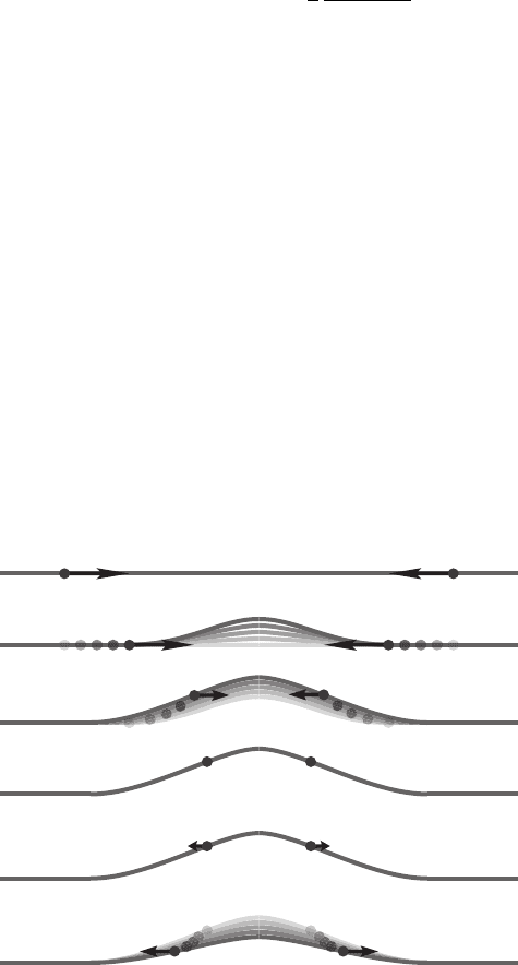
crossings (see Figure 22.1).

Anumerical simulation which does not reproduce the derivatives on a microscopic

level is not sensitive to bumps. Thus it does not prevent the crossing of grid point

trajectories. Also the time step has to be chosen sufﬁciently small, at least a few

times smaller than the distance of two approaching grid points divided by the relative

Bohmian velocity. Otherwise there might not be enough iterations for the quantum

potential to decelerate the approaching grid points.

Things can go wrong in particular when R(q, t) is very small: a small value of

R(q, t) can cause a large quantum potential (Equation 22.9) and therefore large accel-

erations resulting in large velocities.

Typical situations where R(q, t) is small are “nodes” and “tails” of the wavefunc-

tion. Nodes are local zeros of the wavefunction and tails are extended regions in

1. Two grid points which

approach each othert

2. Formation of a

microscopic bump in |ψ|

3. e quantum

potential recognizes this

increase in curvature

4. e grid points are

decellerated

5. In an extreme case the

grid points may pick up

velocities in opposite

direction

6. e curvature of |ψ|

relaxes again

FIGURE 22.1 Deceleration of approaching conﬁguration space trajectories.

Bohmian Grids and the Numerics of Schrödinger Evolutions 351

conﬁguration space where the wavefunction is small. For example one typically has

tails near the boundary of the grid.Asmall numerical error there can cause erroneously

huge quantum potentials because the denominator in Equation 22.9 goes to zero. Note

that this problem is of a conceptual kind since at the boundary there is a generic lack

of knowledge of how the derivatives of R or S in Equations 22.5 through 22.7 behave;

see Figure 22.2 for two example methods of ﬁttings which will be explained later on

in more detail.

We describe brieﬂy how this conceptual problem can cause severe numerical insta-

bility: For this suppose that only the last grid point in the upper left plot of Figure 22.2

is lifted a little bit upwards by, e.g., some numerical error. Then the resulting quan-

0.1

0.05

–0.05

–0.1

0.1

0.05

–0.05

–0.1

–1 –0.5

(a) (b)

(c)

(d)

Analytic function

Fitting polynomial

Grid points used for fitting

Second derivative

Analytic function

Fitting polynomial

Grid point used for fitting

Second derivative

Analytic function

Fitting polynomial

Grid points used for fitting

Second derivative

Analytic function

Fitting polynomial

Grid points used for fitting

Second derivative

0.5 1

0.1

0.05

–0.05

–0.1

–1 –0.5 0 0.5 1

0.1

0.05

–0.05

–0.1

–1 –0.5 0 0.5 1

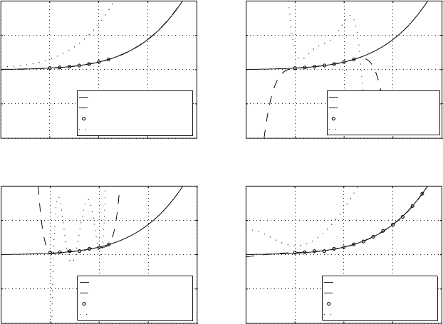
FIGURE 22.2 Fitting a polynomial of sixth degree and its second derivative near the bound-

ary. Upper left: the function to ﬁt smoothly decays. Both least squares and polynomial ﬁtting

give identical ﬁtting polynomials mimicking this decay. Upper right: polynomial ﬁtting was

used while the function value at the fourth grid point was shifted upwards by 10

−4

(not visible

in the plot) to simulate a numerical error in order to see how sensitive polynomial ﬁtting reacts

to such an error. Lower left: all values at the grid points were shifted by an individual random

amount of the order of 10

−3

and polynomial ﬁtting was used. Lower right: all values at the

grid points were shifted by the same random numbers as on the lower left while the additional

grid points were also shifted by individual random amounts of the order of 10

−3

and least

squares ﬁtting was used. By comparison with upper left plot one observes the robustness of

least squares ﬁtting to such numerical errors at the boundary.

352 Quantum Trajectories

tum potential will cause the last grid point to move toward the second last one. This

increases the density of grid points and thus again increases R in the next step such

that this effect is self-amplifying (in fact growing super-exponentially) and will affect

the whole wavefunction quickly.

22.3 FITTING ALGORITHMS: WHAT THEY CAN

DO AND WHAT THEY CAN’T

In the following we shall explain strategies to circumvent the aforementioned prob-

lems of numerical implementations of Bob Wyatt’s idea. As said, in order to perform

the numerical integration the only crucial part in this is computing the derivatives

involved in the set of differential equations. There are several techniques known and

Wyatt [6] gives a comprehensive overview. One technique called least squares ﬁtting

is commonly used. This technique turns out to be numerically stable, however, it can

be inappropriate with respect to the issues discussed in Section 22.2 and thus gives

large numerical errors for general initial conditions and potentials.

On the other hand there are several other ﬁtting techniques, among them polyno-

mial ﬁtting. The latter turns out to give very accurate numerical results in the ﬁrst few

time integration steps, however, it soon becomes unstable. Understanding the source

of instabilities, however, makes it possible to stabilize polynomial ﬁtting.

Fitting Methods. Let us quickly explain the two ﬁtting methods used to compute

the derivatives encountered in Equations 22.5 through 22.7 in the later numerical

example: least squares ﬁtting and polynomial ﬁtting. Both provide an algorithm for

ﬁnding, e.g., a polynomial

∗

of degree, say (m − 1), which is in some sense to be

speciﬁed close to a given function f : R → R known only on a set of, say n, pairwise

distinct data points, (x

, f (x

))

1≤i≤n

, as a subset of the graph of f . The derivative

can then be computed from the ﬁtting polynomial by algebraic means. For the further

discussion we deﬁne

y:=(f (x

))

1≤i≤n

X:=(x

(j −1)

)

1≤i≤n,1≤j ≤m

a = (a

)

1≤i≤m

∈ R

δ = (δ

)

1≤i≤n

∈ R

Using this notation the problem of ﬁnding a ﬁtting polynomial to f on the basis of n

pairwise distinct data points of the graph of f reduces to ﬁnding the coefﬁcients of

the vector a obeying the equation

y = X · a + δ

such that the error term δ is in some sense small. Here the dot · denotes matrix

multiplication. The ﬁtting polynomial is given by p(x) =



j=1

j−1

∗

Or more general an element of an m-dimensional vector space of functions. The coefﬁcients of the design

matrix X determine which basis functions are used.

Bohmian Grids and the Numerics of Schrödinger Evolutions 353

• Polynomial Fitting: For the case n = m we can choose the error term δ to

be identically zero since X is an invertible square matrix and a = X

−1

· y

can be straightforwardly computed.

• Least Squares Fitting: For arbitrary n>mthere is no longer a unique

solution and one needs a new criterion for ﬁnding a unique vector a. The

algorithm of least squares ﬁtting therefore uses the minimum value of the

accumulated error ∆ :=



i=1

w(x − x

)δ

where w : R → R speciﬁes a

weight dependent on the distance between the i-th data point x

and some

point x where the ﬁtting polynomial is to be evaluated. The vector a can

now be determined by minimizing ∆ as a function of a by solving



∂∆(a)

∂a



1≤j≤m



−2



i=1

w(x − x

)(y −X · a)

j−1



1≤j≤m

= 0.

Note that for m = n and any non-zero weight w the algorithm of least

squares ﬁtting produces the same a as the polynomial ﬁtting would do since

for a determined by polynomial ﬁtting the non-negative function ∆(a)is

zero and thus a naturally minimizes the error term.

The advantage of polynomial ﬁtting is that the ﬁtting polynomials actually go

through all the data points, (x

, f (x

))

1≤i≤n

. However, when data points lie unfavor-

ably the resulting ﬁtting polynomial may have high oscillations, see e.g., Figure 22.2.

The advantage of least squares ﬁtting is that it produces very smooth ﬁtting poly-

nomials. However, the ﬁtting polynomials do not reproduce the derivatives of f on

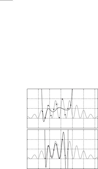
the scale of the grid points, see e.g., Figure 22.3.

Least square fitting

Exact polynomial fitting

FIGURE 22.3 Comparison of least squares ﬁtting and polynomial ﬁtting. The stars denote

the data points used for the ﬁtting, the red function denotes the wavefunction to be ﬁtted and

the blue function denotes the ﬁtting polynomials. Note that the least squares ﬁtting polynomial

does not even reproduce the correct sign of the derivative at the marked point.