Chattaraj P.K. (Ed.) Quantum Trajectories

Подождите немного. Документ загружается.

314 Quantum Trajectories

(0), P

(0)

(t), P

(t)

(a)

ψ(t)ψ(0)

(t) e

(b)

ψ(t)ψ(0)

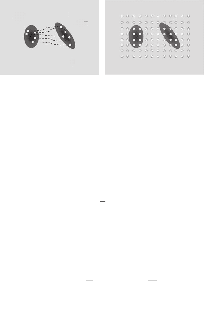
FIGURE 20.1 Random trajectory guided grid (a) versus regular basis covering the whole

dynamically important space (b).

20.2 THEORY

20.2.1 VARIATIONAL PRINCIPLE

First we consider a general derivation of the quantum equations of motion. It is well

known that the time dependence of a wavefunction Ψ(α

, α

, ...,α

) is simply that

of its parameters, and the equations for the “trajectories” α

(t) can be worked out

from the variational principle

δS = 0 (20.1)

by minimizing the action S =



Ldt of the Lagrangian

∗

, ...,

∗

, α

∗

, ...,α

∗

, ...,

, α

, ...,α

)

Ψ(α

∗

, α

∗

, ...,α

∗

)

∂

∂t

−

Ψ(α

, α

, ...,α

)

. (20.2)

The variational principle Equation 20.1 straightforwardly leads to the Lagrange equa-

tions of motion

∂L

∂α

−

∂L

∂

= 0, (20.3)

and an adjoint equation for the complex conjugate, where α is the complex vector of

wavefunction parameters α ={α

, α

, ...,α

After introduction of the momentum p ={p

, p

, ...,p

}

(α

∗

, ...,α

∗

, α

, ...,α

) = 2

∂L

∂

= i



∗

, ...,α

∗



∂

∂α

Ψ(α

, ...,α

)

(20.4)

the Lagrange Equation 20.3 can be written in the Hamilton form

∂H 

∂p



∂H 

∂α

∗

∂α

∗

∂p

(20.5)

Trajectory Guided Grids of Coherent States 315

where the Hamiltonian



H =Ψ(α

∗

, α

∗

, ...,α

∗

H |Ψ(α

, α

, ...,α

) (20.6)

is not an explicit function of the momenta (Equation 20.6). This is the reason why

the derivative of the Hamiltonian with respect to the momentum is expressed through

the derivatives with respect to α and the unknown matrix ∂α

∗

/∂p

= (D

−1

)

which

must be obtained by inverting

∂p

∂α

∗

= i

∂

∂α

∗

Ψ(α

∗

, α

∗

, ...,α

∗

)

∂

∂α

(

, α

, ...,α

)

. (20.7)

In other words Hamilton’s equations can be written as a system of linear equations

for the derivatives of the wavefunction parameters

α =

∂H 

∂α

. (20.8)

Equations 20.3 and 20.8 are the main result of the work of Kramer and Saraceno [4].

Although variational principle is well known and its applications to the grids of

Gaussian wavepackets can be traced back to the work of Metiu and coworkers [5],

the approach of [4] is perhaps the most elegant way to derive the equations of quantum

mechanics.

In the simplest case of the wavefunction presented as a superposition of orthonor-

mal basis functions

|Ψ=



i=1,N

|ϕ

, (20.9)

so that α = a ={a

, ...,a

}, the matrix D is simply a unit matrix, and the Kramer–

Saraceno Equations 20.3, 20.8 yield the standard Schrödinger equation in the form

of coupled equations for the amplitudes

a = Ha (20.10)

where H is the matrix of the Hamiltonian. However, in many cases, for example in

the case of Gaussian coherent state basis sets, the D-matrix is not diagonal and the

system of linear Equation 20.8 for the derivatives has to be resolved at each step of

the propagation.

20.2.2 V

ARIATIONAL MULTICONFIGURATIONAL GAUSSIANS (vMCG)

Although the equations of time-dependent quantum mechanics for the wavefunction

Equation 20.9, which uses a simple orthonormal basis, are very simple, Equation 20.10

can be used for systems with only a few degrees of freedom (DOF) because the size

of the basis set N grows exponentially with the number of DOF. For multidimen-

sional systems trajectory guided random basis sets can be more efﬁcient. The main

idea of the vMCG technique, which is an all-Gaussian version of the more general

G-MCTDH method [1], is to apply the variational principle to the wavefunction which

316 Quantum Trajectories

is represented by a superposition of frozen Gaussian wavepackets also called coherent

states (CS)

|Ψ=



l=1,N

(t)|z

(t). (20.11)

The coherent state represents a phase space point “dressed” with the ﬁnite width of

the wavepacket determined by the parameter γ = mω/. For notational simplicity

everywhere in this chapter it is assumed that the units are such that the Planck con-

stant  and the width parameter γ are equal to one. A multidimensional CS includes

coordinates and momenta of all M DOF |z

=|z

(1)

···|z

(M)

. In the coordinate

representation coherent states are Gaussian wavepackets

x|z=





exp



−

(x −q)



p(x − q) +

ipq

2



(20.12)

where q is the position of the wavepacket, its classical momentum p is given by

z =

q +i

−1

−

√

∗

q −i

−1

−

√

(20.13)

and Equation 20.12, written for a one-dimensional CS, can easily be generalized to

many dimensions.

An important property of the wavefunction Equation 20.11 is that the basis CSs

are not orthogonal. The overlap is given as

z

=Ω

= exp



∗

−

∗

−

∗



. (20.14)

If |z is a multidimensional CS then the parameters of the M-dimensional wave-

function Equation 20.11 are the N amplitudes a

i=1,...,N

and the N × M com-

plex parameters z

(m=1···M)

l=1···N

of the CS basis functions |z

=|z

(1)

···|z

(M)

, i.e.,

α ={a

, ...,a

, z

(1)

, ...z

(1)

, ...,z

(M)

, ...z

(M)

}. As has been shown in Ref. [6]

the equations of vMCG are those of Kramer and Saraceno theory applied to the

wavefunction Equation 20.11. Due to the apparent complexity and length of the

vMCG equations they are not given in the main body of this chapter but are pre-

sented in the Appendix instead. However, the vMCG theory simply relies on the

Kramer–Saraceno system of linear equations for the derivatives of the wavefunction

parameters. Numerical solution of the vMCG equations is quite demanding. It requires

ﬁnding the derivatives of the wavefunction parameters by resolving the linear system

of size N ×M +N at each time step.

20.2.3 V

ARIATIONAL SINGLE CONFIGURATIONAL GAUSSIAN (vSCG)

There is one case, however, when the solution of the vMCG equations can easily

be obtained, which is when the wavefunction Equation 20.11 contains only a single

conﬁguration (N = 1)

|Ψ=a|z. (20.15)

Trajectory Guided Grids of Coherent States 317

The equations for the derivatives of z and a become

z =−i

∂z|

H |z

∂z

∗

(20.16)

and

−i ˙a =



∗

−

∗

−z|

H |z



a. (20.17)

The solution of Equation 20.16 yields a trajectory z(t) in the Hamiltonian which

is quantum averaged over the wavepacket z. The solution of Equation 20.17 is very

simple. It is made up of a constant prefactor multiplied by the exponent of the classical

action

a = a(0) exp(iS) (20.18)

where

S =





∗

−

∗

−z|

H |z



dt. (20.19)

The fact that the evolution of a single frozen Gaussian CS is given by the trajectory

(Equation 20.16) and the amplitude Equation 20.18 as a product of a constant prefactor

and the exponent of the classical action along the trajectory, has been well known

since the famous work of Heller on the frozen Gaussian approximation [7].

20.2.4 C

OUPLED COHERENT STATES (CCS)

The method of CCS [2] attempts to decrease the computational cost of vMCG. The

CCS technique uses exactly the same form of the wavefunction Equation 20.11 as

vMCG with the difference that the CCS method does not ﬁnd the trajectories of

the coherent states z from the full variational principle. Instead the trajectories are

taken in the form Equation 20.16 which is “optimal” for a single CS wavefunction

Equation 20.15. Only the equations for the amplitudes are obtained from the full

variational principle.

In the CCS approach the equations for the amplitudes

iΩE

d = ∆



Ed (20.20)

are usually written for the preexponential factor so that in the expression for the

wavefunction the oscillating exponent is factored out of the amplitude

|Ψ(t)=



(t)e

(t)

(t). (20.21)

In Equation 20.20 Ω is the overlap matrix and E is the diagonal matrix of classical

action exponents E

= e

and ∆



is a matrix which includes the Hamiltonian.

See Ref. [2] and the Appendix for more details.

318 Quantum Trajectories

Assuming the trajectories, instead of getting them from the full variational prin-

ciple, results in huge computational savings. Only the system of N equations for the

derivatives of the coupled amplitudes has to be solved comparably to the N ×M +N

size of the linear system in the vMCG technique. As a result CCS can afford a much

larger basis set. Making assumptions about the trajectories is not an approximation

but simply a reasonable choice of time-dependent basis set because the variational

principle is still applied to the amplitudes of the basis CSs. The price which CCS pays

for its efﬁciency is that the trajectories of the basis CS are not as ﬂexible as in vMCG.

Nevertheless as has been shown in many instances the CCS method is capable of

accurate treatment of quantum multidimensional systems.

20.2.5 T

HE GAUSSIAN MULTICONFIGURATIONAL TIME-DEPENDENT HARTREE METHOD

Many problems of quantum mechanics naturally require regular basis sets for a few of

the most important DOF, but a grid of randomly selected trajectory guided Gaussians

for the rest of the DOF. For example, a description of nonadiabatic transitions between

two or more potential energy surfaces can be done with the help of the following

multiconﬁgurational wavefunction anzats:

|Ψ(t)=



k=1,N

(t)|ϕ

+a

(t)|ϕ

)|z

(t). (20.22)

In each conﬁguration |ϕ

 and |ϕ

 represent a regular basis for the two elec-

tronic states and |z

(t) is a CS describing the nuclear DOF. Another example is

the so-called system-bath problems where a small subsystem is treated on a regular

basis set or grid and a random grid of Gaussians is used to describe a large num-

ber of the harmonic bath modes. Applying the Kramer and Saraceno approach in

its Lagrange Equation 20.3 or Hamiltonian Equation 20.8 form to the parameters

of the wavefunction Equation 20.22 would give the equations of the G-MCTDH

method [3] in their simplest form, which again can be written as a system of linear

equations for the time-dependent derivatives of the wavefunction parameters.

∗

Fully

variational G-MCTDH equations for the vector α = (a

, ...,a

, a

, ...,a

, ...,z

, z

, ...,z

) of the parameters of the wavefunction Equation 20.20

are given in the Appendix.

20.2.6 T

HE EHRENFEST METHOD

The equations of G-MCTDH simplify when the wavefunction Equation 20.20

includes only one conﬁguration

|Ψ(t)=(a

(t)|ϕ

+a

(t)|ϕ

+···)|z(t). (20.23)

As has been shown in Ref. [4] the equations for the parameters of the wavefunction

Equation 20.21 become those of the Ehrenfest dynamics [8]

∗

Although G-MCTDH allows more sophisticated ways of presenting the “system” part of the wavefunc-

tion, for simplicity only the form Equation 20.22 is considered here. Generalization is not too difﬁcult.

Trajectory Guided Grids of Coherent States 319

˙a

= i



∗

−

∗

− H



− iH

(20.24)

˙a

= i



∗

−

∗

− H



− iH

(20.25)

for the amplitudes of “system” states along the trajectory of the “bath”

z =−

∂H

Ehr

∂z

∗

(20.26)

where

Ehr

=Ψ|

H |Ψ=

∗

+ H

∗

+ H

∗

+ H

∗

+ a

∗

(20.27)

is the Ehrenfest Hamiltonian, which is the Hamiltonian of the “bath” averaged over

the quantum wavefunction of the “system.”

Similar to the CCS theory it is convenient to write the solution for the amplitudes

as a product of the oscillating exponent of the classical action and a relatively smooth

preexponential factor a

1,2

= d

1,2

exp(iS

1,2

), for which Equations 20.24 become

=−iH

exp(i(S

− S

)) (20.28)

=−iH

exp(i(S

− S

)). (20.29)

Equations 20.24 through 20.27 represent the well-known Ehrenfest approach [8]

which treats the system with a set of basis functions |ϕ

, |ϕ

, . . . and the bath with

a single trajectory |z(t ).

20.2.7 T

HE MULTICONFIGURATIONAL EHRENFEST METHOD

In Ref. [4] a method called Multiconﬁgurational Ehrenfest dynamics has been sug-

gested. Similar to the G-MCTDH technique it uses a formally exact anzats Equa-

tion 20.22, which converges to the exact wavefunction, but the difference is that the

CS positions z(t ) are not considered as variational parameters. Instead the trajectories

z(t ) are chosen from Equations 20.25, 20.26 of the Ehrenfest method. Only the lin-

ear system Equation A.3 for the time derivatives of the amplitudes is obtained from

the full variational principle and should be resolved. This results in a huge gain in

computational efﬁciency. Only the system of 2N equations for the derivatives of the

coupled amplitudes has to be solved comparably to the N ×M +2N size of the system

Equations 20.3, 20.8 in the G-MCTDH technique. Just like in the case of the CCS

method, making assumptions about the trajectories is not an approximation but simply

a reasonable choice of a time-dependent basis set because the variational principle

is still applied to the amplitudes. Reference [4] reports simulations of the spin-boson

model with up to 2000 DOF, which is among the biggest quantum systems for which

the Schrödinger equation has ever been solved numerically without approximations.

320 Quantum Trajectories

20.3 CONCLUSIONS

This chapter has shown that

(1) The equations of the vMCG and G-MCTDH techniques can be obtained as

those of Kramer–Saraceno theory for multiconﬁgurational wavefunction.

(2) Heller’s frozen Gaussian and Ehrenfest dynamics also follow from the

Kramer–Saraceno approach applied to a single conﬁguration wavefunction

only.

(3) The method of CCS combines the trajectories of HFG with the vMCG equa-

tions for the amplitudes.

(4) The MCE technique uses Ehrenfest trajectories with G-MCTDH coupled

equations for the amplitudes

(5) The advantage of CCS and MCE is that they reduce dramatically the number

of linear equations for the time derivatives of the wavefunction parameters.

(6) Using “approximate” trajectories instead of those yielded by a fully vari-

ational approach is not an approximation but simply a choice of basis set.

The choice of CCS and MCE is efﬁcient but may be less ﬂexible than that

of the vMCG and G-MCTDH methods.

APPENDIX: VARIATIONAL PRINCIPLE AND THE EQUATIONS

OF G-MCTDH

The variational principle has been applied to the derivation of equations for many types

of wavefunction parametrization. For example, recently we analyzed the equations of

motions for the parameters of the wavefunctions represented as a superposition of

Gaussian coherent states [6]. To obtain the Lagrangian Equation 20.2 one should

notice that

∂

∂t





∂

∂t

−



∂

∂t



where the operators



∂

∂t

and



∂

∂t

act on the left and on the right. Then

∗

∂

∂t

= a

∗





∂

∂t

−



∂

∂t



(A.1)

∗˙a

− a

˙a

∗]z





∗

−

∗

−

∗



−



∗−

∗

−

∗



∗ a

z

.

Trajectory Guided Grids of Coherent States 321

To perform differentiation over time in Equation A.1 one must use the formula Equa-

tion 20.14 for the CS overlap. Then the Lagrangian becomes

L =

∂

∂t

−



∗

˙a

−˙a

∗

]z







∗

−

∗

−

∗



−



∗

−

∗

−

∗





∗

z





∗

˙a

−˙a

˙a

∗

]z







∗

−

∗

−

∗



−



∗

−

∗

−

∗





∗

z





z

a

∗

−



z

a

∗

−



z

a

∗

−



z

a

∗

. (A.2)

The Lagrange equations for the amplitudes are



i ˙a

z

−z

a

−z

a

+ i



∗

− z

∗

)

∗

−

∗



z

a

= 0 (A.3)

and similarly for a

. It is convenient to modify Equation A.2 by writing the ampli-

tudes as a product of the oscillating exponent of the classical action and a smooth

preexponential factor a

(t) = d

(t)e

(t)

and a

(t) = d

(t)e

(t)

and using the

equations for d instead of Equation A.2, which are



z

=



∆



∗

, z



z

d

(A.4)

and similarly for d

. In Equation A.4

∆



=[z

−z

z

−iz

(z

∗

− z

∗

)

] (A.5)

are the elements of the matrix ∆



in Equation 20.20. The variation of z parameters

yields

322 Quantum Trajectories

∗







−

∂H

∗

, z

)

∂z

∗



+ a



−

∂H

∗

, z

)

∂z

∗

!

z



+ a

∗



i ˙a

− z

)z



+ a

∗



− z

)z



∗

− z

∗

)

∗

−

∗



− H

∗

, z

)

+ a

∗







−

∂H

∗

, z

)

∂z

∗



+ a



−

∂H

∗

, z

)

∂z

∗

!

z



+ a

∗



i ˙a

− z

)z



+ a

∗



− z

)z



∗

− z

∗

)

∗

−

∗



− H

∗

, z

)

= 0. (A.6)

Although they look complicated, Equations A.6 are simply a system of linear equa-

tions for the derivatives of z. Together with Equations A.3 for the derivatives of the

amplitudes they constitute the system of Kramer–Saraceno equations D

α = ∂H /∂α

for the full variation of parameters. They are equivalent to those of the G-MCTDH

method also based on the full variational principle. Solving the full system Equa-

tionsA.3,A.6 for 2N amplitudes together with the N ×M parameters z is an expensive

computational task. The central idea of the MCE approach is to use predetermined

trajectories which are close to the solution of Equation A.6. If the coherent states |z



and |z

 are far away from each other then their overlap is small and all nondiago-

nal terms in Equation A.6 can be neglected. Then Equation A.6 becomes that of the

individual CS Equation 20.23.

MCE uses trajectories other than those yielded by the full variational principle,

but it is still a fully quantum approach, which is formally exact and can converge to

accurate quantum result. This proves that the choice of Ehrenfest trajectories to guide

the grid is a good one.

The vMCG equations are those of G-MCTDH Equation A.3, Equation A.6 but for

a single function |ϕ

and therefore can be obtained from EquationA.3, Equation A.6

simply by dropping all terms containing the index “2”. CCS is obtained from MCE

in a similar fashion.

BIBLIOGRAPHY

1. I. Burghardt, H.D. Meyer, and L.S. Cederbaum, J. Chem. Phys., 111, 2927 (1999); G.A.

Worth and I. Burghardt, Chem. Phys. Lett., 368, 502 (2003); I. Burghardt, M. Nest, and

G.A. Worth, J. Chem. Phys., 119, 5364 (2003); I. Burghardt, K. Giri, and G.A. Worth,

J. Chem. Phys., 129 174101 (2008).

Trajectory Guided Grids of Coherent States 323

2. D.V. Shalashilin and M.S. Child, J. Chem. Phys., 113, 10028 (2000); D.V. Shalashilin and

M.S. Child, J. Chem. Phys., 114, 9296 (2001); D.V. Shalashilin and M.S. Child, J. Chem.

Phys., 115, 5367 (2001); D.V. Shalashilin and M.S. Child, J. Chem. Phys., 121, 3563

(2004); P.A.J. Sherratt, D.V. Shalashilin, and M.S. Child, Chem. Phys., 322, 127 (2006);

D.V. Shalashilin and M.S. Child, Chem. Phys., 304, 103 (2004).

3. D.V. Shalashilin, J. Chem. Phys., 130 244101 (2009).

4. P. Kramer and M. Saraceno, Geometry of the Time-Dependent Variational Principle in

Quantum Mechanics (Springer, New York, 1981).

5. S.I. Sawada, R. Heather, B. Jackson, and H. Metiu, J. Chem. Phys., 83 3009 (1985);

S.I. Sawada, H. Metiu, J. Chem. Phys., 84 227 (1986).

6. D.V. Shalashilin and I. Burghardt, J. Chem. Phys., 129, 084104 (2008).

7. E.J. Heller, J. Chem. Phys., 75, 2923 (1981).

8. G.D. Billing, Chem. Phys. Lett., 100, 535 (1983); H.-D. Meyer and W.H. Miller, J. Chem.

Phys., 70, 314 (1979).