Chattaraj P.K. (Ed.) Quantum Trajectories

Подождите немного. Документ загружается.

Direct Numerical

Solution of the Quantum

Hydrodynamic Equations

of Motion

Brian K. Kendrick

CONTENTS

21.1 Introduction.................................................................................................325

21.2 The Quantum Hydrodynamic Equations of Motion ...................................328

21.3 The MLS/ALE Method...............................................................................329

21.4 Example Scattering Problems Using the MLS/ALE Method.....................331

21.4.1 One to Four-Dimensional Scattering Off an Eckart Barrier .........331

21.4.2 One-Dimensional Scattering Off a Rounded Square Barrier........334

21.4.3 DynamicalApproximations for Treating Quantum Many-Body

Systems.........................................................................................337

21.5 The Iterative Finite Difference Method ......................................................339

21.6 Concluding Remarks and Future Research.................................................342

Acknowledgments..................................................................................................343

Bibliography ..........................................................................................................343

21.1 INTRODUCTION

The quantum hydrodynamic formulation of quantum mechanics is intuitively appeal-

ing [1–7]. The quantum potential (Q) and its associated force f

=−∇Q appear

on an equal footing with the classical potential and force in the equations of motion.

Thus, this approach provides a uniﬁed computational method for including both clas-

sical and quantum mechanical effects in a molecular dynamics (trajectory based)

calculation. However, despite their deceptively simple form, the quantum hydrody-

namic equations of motion are very challenging to solve numerically. The quantum

potential is non-local (i.e., the trajectories are coupled) and it is a non-linear func-

tion of the density (i.e., it depends upon the solution itself). Thus, unlike a typical

classical potential, the quantum potential is manifestly time dependent and evolves

in “lock-step” fashion with the dynamics. Furthermore, the quantum potential can

325

326 Quantum Trajectories

often become singular when “nodes” occur in the quantum mechanical wave func-

tion. The problematic nodes are often associated with quantum interference effects

due to the reﬂected components of the wave function scattering off a potential barrier.

Despite these formidable challenges, signiﬁcant progress has been made in recent

years addressing each of the issues mentioned above.

The direct numerical solution methods can be split into three categories based

on the underlying reference frame: (1) Lagrangian, (2) Eulerian, and (3) Arbitrary

Lagrangian–Eulerian (ALE). The ﬁrst successful direct numerical solution method

for solving the quantum hydrodynamic equations, called the Quantum Trajectory

Method (QTM), was based on the Lagrangian frame of reference [8]. One advantage

of the Lagrangian frame is the simpliﬁed equations of motion due to the computational

grid moving with the ﬂuid ﬂow. Another advantage is the grid being optimal. That is,

the grid points move with and follow the time evolution of the density so that there are

few wasted grid points located in regions where the density is small or zero. However,

there is a signiﬁcant disadvantage associated with using a Lagrangian frame. As time

evolves, the grid becomes highly non-uniform which makes an accurate evaluation

of the numerical derivatives difﬁcult. Unfortunately, the grid often becomes sparse

in precisely the regions where more grid points are needed for accurate calculations

(i.e., near impending node formation) [9]. The Eulerian grid has the advantage of

using a ﬁxed grid that does not change with time. Thus, the grid remains uniform

as time evolves and the sparsity of grid points near nodes is avoided. Unfortunately,

the number of grid points is typically much larger since the entire computational

domain must be gridded and included in the calculations from the beginning. However,

in practice, the Eulerian grid size problem can be mitigated by “deactivating” grid

points with small density and then “activating” them as the density increases above

some user speciﬁed threshold during the calculation (some care is required in order

to ensure continuity in the solutions when initializing all of the ﬁeld values at the

newly activated grid points). As the name implies, the ALE frame combines the best

properties of both the Lagrangian and Eulerian frames of reference [10]. An ALE

frame can be constructed which follows the ﬂow of the ﬂuid while preserving a

uniform grid spacing. By implementing automatic grid reﬁnement, a nearly constant

user speciﬁed grid spacing can also be maintained [11].

Within each of the three frames of reference discussed above, a given numerical

approach can be further subdivided into its method for evaluating derivatives and

propagating in time. One of the most successful methods for evaluating derivatives

within the quantum hydrodynamic approach is the meshless Moving Least Squares

(MLS) method [8, 11]. This approach has been most successful due largely to its

“noise ﬁltering” properties. In the MLS approach, the derivatives of a ﬁeld are simply

the coefﬁcients of a local polynomial ﬁt to the ﬁeld values within some local radius of

the desired evaluation point. The local least squares ﬁtting tends to average out any

noise or numerical errors which may be accumulating in the solution which helps to

stabilize the calculations. On the other hand, the ﬁltering also reduces the resolution

or ﬁdelity of the calculations. Unfortunately, the accuracy, stability, and convergence

properties of the MLS approach are not well understood which can make it difﬁcult

to use in practice. Furthermore, the derivatives are not strictly continuous due to the

different local neighborhoods used at each evaluation point. Also, the computational

Numerical Solution of the Quantum Hydrodynamic Equations 327

overhead associated with performing repeated local least squares ﬁts often becomes

signiﬁcant. Mesh based approaches can also be used for evaluating derivatives such

as ﬁnite differences and ﬁnite elements. The advantages of ﬁnite differences include

ease of implementation, computational efﬁciency, higher resolution/ﬁdelity, and con-

tinuous derivatives (to some speciﬁed order). The accuracy, stability and convergence

properties of ﬁnite difference approximations are much better understood relative to

the meshless MLS approach. Until recently, ﬁnite difference based approaches for

solving the quantum hydrodynamic equations of motion have been plagued with insta-

bilities. These instabilities have recently been shown to originate from the negative

diffusion terms associated with the truncation error of a ﬁnite difference approxima-

tion to the quantum hydrodynamic equations [12]. By deriving the explicit analytic

form of these negative diffusion terms, a stabilizing positive diffusion term can be

introduced (called “artiﬁcial viscosity”) which is of the same order as the errors asso-

ciated with the ﬁnite difference approximation [13]. Thus, the stability of the method

can be maintained as the resolution of the calculation is increased.

In any computational method, there are always inherent numerical approximations

such as: grid spacing, time step, polynomial basis set size, etc. We refer to these as

“numerical approximations.” Other kinds of approximations which simplify or reduce

the computational complexity of the original dynamical equations can also be made

such as: incompressible ﬂow, decoupling approximations (i.e., ignoring certain cou-

pling terms), etc. We refer to these as “dynamical approximations.” The difference

between the numerical and dynamical approximations is that the errors associated

with the numerical approximations can be reduced (via grid reﬁnement for example)

to any desired level, whereas the errors associated with a dynamical approximation

are always present (since the original equations have been modiﬁed). In practice,

a combination of both numerical and dynamical approximations is usually required

in order to obtain a computationally feasible method (especially for systems with

many degrees of freedom). In this work the focus will be primarily on the numerical

approximations but a few dynamical approximations will be discussed as well.

The relevant hydrodynamic equations of motion are introduced in Section 21.2. A

meshless numerical solution method based on an ALE frame of reference and MLS

ﬁtting will be reviewed in Section 21.3. This method employs automatic grid reﬁne-

ment, ﬁeld averaging, and artiﬁcial viscosity in order to obtain accurate and stable

propagation for long times. The results of example calculations for a one- and two-

dimensional (2D) Gaussian wave packet scattering off an Eckart potential barrier

will be presented in Section 21.4.1. A generalized artiﬁcial viscosity algorithm will

be reviewed in Section 21.4.2. This method is based on “dynamic” artiﬁcial viscos-

ity coefﬁcients which increase and decrease automatically depending upon the local

strength of the quantum force (i.e., near impending nodes). The results of a challeng-

ing example calculation using this approach to treat a quantum resonance will be

presented. A dynamical approximation (the Vibrational Decoupling Scheme [VDS])

will be reviewed in Section 21.4.3. In this approach, the trajectories associated with

bound vibrational degrees of freedom are decoupled which allows for linear scaling

of the computational cost. Scattering results will be presented for an N -dimensional

Gaussian wave packet tunneling through an Eckart barrier along a reaction path cou-

pled to N − 1 harmonic oscillator (bath) degrees of freedom (for values of N up to

328 Quantum Trajectories

N = 100). The recently developed Iterative Finite Difference Method (IFDM) will be

reviewed in Section 21.5. This grid based approach is a promising alternative to using

a meshless MLS method for evaluating derivatives. The numerical errors and stability

properties of the IFDM are better understood and controllable. One-dimensional scat-

tering results based on the IFDM will be presented. Concluding remarks and future

research directions will be summarized in Section 21.6.

21.2 THE QUANTUM HYDRODYNAMIC

EQUATIONS OF MOTION

In the de Broglie–Bohm approach, the wave function is written in polar form

ψ(r, t ) = R(r, t) exp(iS(r, t)/) where R and S are the real-valued amplitude and

action function. Substituting this expression for ψ into the time dependent Schrödinger

equation and separating into real and imaginary parts gives rise to the following two

equations [1–7]

∂ρ(r, t)

∂t

+∇·



∇S



= 0 , (21.1)

−

∂S(r, t)

∂t

|∇S|

+ V (r) + Q(r, t) , (21.2)

where the probability density ρ(r, t) ≡ R(r, t )

, m is the mass, and V is the interaction

potential. The velocity and ﬂux are deﬁned as v(r, t) =∇S/m and j = ρ v, respec-

tively. Equation 21.1 is recognized as the continuity equation and Equation 21.2 is

the quantum Hamilton–Jacobi equation. Equation 21.2 is identical to the classical

Hamilton–Jacobi equation except for the last term involving the quantum potential

Q which is deﬁned as

Q(r, t ) =−



∇

R =−



−1/2

∇

1/2

. (21.3)

Equation 21.3 shows that Q depends upon the shape or curvature of ψ, and that it can

become singular whenever R → 0. The quantum potential gives rise to all quantum

effects (i.e., tunneling, zero-point energy, etc.). Numerically it is more efﬁcient to

work with the C-amplitude given by R = e

. In terms of C, Equation 21.3 becomes

Q =−



(∇

C +|∇C|

) . (21.4)

The total time derivative in an ALE frame of reference is d/dt = ∂/∂t +

r ·∇

where the grid point velocity

r is not necessarily equal to the ﬂow velocity v.Inan

ALE frame of reference and using ρ = e

, Equations 21.1 and 21.2 become

dC(r, t)

=−

∇·v + (

r −v) ·∇C , (21.5)

dS(r, t)

= L

+ (

r −v) · (mv) , (21.6)

Numerical Solution of the Quantum Hydrodynamic Equations 329

where L

is the quantum Lagrangian deﬁned as

m|v|

− (V (r) +Q(r, t)) . (21.7)

Taking the gradient of Equation 21.2 leads to the familiar equation of motion which

in an ALE frame is given by

=−∇(V + Q) +(

r −v) · (m∇v) . (21.8)

The Lagrangian and Eulerian frames correspond to the special cases

r = v and

r = 0, respectively. Equations 21.5 through 21.8 constitute a set of non-linear cou-

pled hydrodynamic (ﬂuid like) equations which describe the “ﬂow” of the quantum

probability density. The ﬂow lines of this “probability ﬂuid” correspond to the quan-

tum trajectories which are obtained by solving the equation

r = v. The quantum

potential is a non-local interaction which couples these trajectories. If the quantum

potential is zero, then these trajectories correspond to an uncoupled ensemble of

classical trajectories. A solution to the set of Equations 21.5 through 21.8 is com-

pletely equivalent to solving the time dependent Schrödinger equation. However,

despite their relatively simple appearance, these equations are notoriously difﬁcult

to solve numerically. Any small numerical error in computing the spacial derivatives

can become quickly ampliﬁed as these equations are propagated in time. Most of the

numerical problems can be traced to the non-linear dependence of Q on C given by

Equation 21.4.

21.3 THE MLS/ALE METHOD

In this section we review the MLS/ALE method for solving the quantum hydrody-

namic equations of motion [11].This approach uses the MLS algorithm for computing

derivatives and an ALE reference frame [10]. The probability ﬂuid is discretized into

n computational particles or ﬂuid elements so that the amplitude C

, action S

, ﬂow

velocity v

, and grid points r

are labeled by i = 1, ...,n. Once the initial conditions

at time t are speciﬁed for all of these ﬁelds at each value of i, the coupled set of quan-

tum hydrodynamic Equations 21.5 through 21.8 are propagated to time t +∆t using

a fourth-order Runge–Kutta time integrator. All of the ﬁelds and their derivatives

which appear in these equations are evaluated using a fourth-order MLS algorithm

(see Ref. [11] for more details). The solutions are monitored for convergence as

the grid spacing and time step are decreased. Special attention must be paid to the

“radius of support” in the MLS algorithm. The radius of support deﬁnes a spherical

neighborhood around a given evaluation point. All points within this local spherical

neighborhood are used in the local least squares ﬁt. As the grid spacing is decreased,

the optimal radius of support also changes. A variable radius support which depends

upon the probability density was found to give the best stability (especially near the

edges of the grid where a larger radius is needed).

The ALE frame requires the user to specify the grid velocities (the ˙r in Equa-

tions 21.5 through 21.8). The idea is to choose these grid velocities in order to

330 Quantum Trajectories

minimize the numerical errors. A uniform grid spacing was found to be most accurate

and can be constructed by choosing the ˙r

to satisfy (in one spacial dimension)

˙r



− r

)

∆t

(21.9)

where t



= t + ∆t. The r



and r

are the particle positions on the uniform grids at

times t



and t, respectively. The uniform grid at the future time step t



is constructed

by ﬁrst performing the time propagation from time t to t



using a Lagrangian frame

(i.e., ˙r = v) in Equations 21.5 through 21.8. A uniform grid is constructed between

the new end points r

and r

by uniformly distributing the n − 2 interior points. The

propagation from time t to t



is then repeated using the ALE frame with the ˙r given

by Equation 21.9. This process is repeated for each time step so that by construction

the ALE grid remains uniform as time evolves. The ALE grid also follows the ﬂow

of probability density since the end points are propagated using a Lagrangian frame

(i.e., the end points move along quantum trajectories). Thus, the grid is optimal in that

only grid points with non-zero density are included in the calculation. However, as

the wave packet spreads, the uniform grid spacing increases. In order to maintain the

resolution of the calculation, an automatic grid reﬁnement algorithm is used which

increases the number of points n → n



= n + ∆n as the calculation progresses. The

number of points added (∆n) is chosen so that the effective grid spacing (r

−r

)/n



remains less than some user speciﬁed value. The MLS algorithm is then used to

interpolate new values of the ﬁelds at the new n



points. The grid reﬁnement is not

done at each time step. A threshold is set so that the grid reﬁnement only occurs

when ∆n>5. The ALE frame with automatic grid reﬁnement produces an optimal,

uniform grid with nearly constant grid spacing as time evolves.

The unitarity of the MLS/ALE method is signiﬁcantly improved by using averaged

ﬁelds. In this approach, the MLS/ALE solution is propagated from time t to t



and all

of the ﬁelds and their derivatives (Q, V , f

, f

, ∇C, ∇·v, and ∇v) are computed at

the future time t



using the fourth-order Runge–Kutta method. These values are then

averaged with their values at the previous time step t . The MLS/ALE solution is then

recomputed from time t to t



using these averaged ﬁelds. In analogy with implicit ﬁnite

differencing, the use of averaged ﬁelds cancels out some of the numerical errors in the

calculation which results in a more accurate solution (i.e., higher order). However,

since the ALE/MLS method is already fourth-order accurate in both space and time,

perhaps a better analogy for using averaged ﬁelds is that it represents the ﬁrst iteration

in a non-linear iterative solution method (see Section 21.5).

In the absence of nodes, the MLS/ALE method with automatic grid reﬁnement and

averaged ﬁelds is an accurate and stable method for the direct numerical solution of

the quantum hydrodynamic equations. However, when nodes begin to occur (due to

the quantum interference associated with the reﬂected components of a wave packet

scattering off a potential barrier for example), the singular nature of Q and f

near

the forming nodes causes the method to break down. Associated with an impending

node is a “kink” in the velocity ﬁeld. As a node forms, this kink develops into a sharp

discontinuity at the node’s location. In classical hydrodynamics, sharp discontinuities

Numerical Solution of the Quantum Hydrodynamic Equations 331

in the velocity ﬁeld are often associated with shock fronts. Thus, quantum interference

can be interpreted as a source of shock fronts within the quantum hydrodynamic

formulation.A standard technique for stabilizing classical hydrodynamic calculations

in the presence of shocks is the introduction of artiﬁcial viscosity [11,13]. Artiﬁcial

viscosity produces a stabilizing force which prevents the negative slope associated

with the kink in the velocity ﬁeld from becoming too large. Thus, the discontinuity

in the velocity ﬁeld is avoided as well as the singularities in Q and f

. In effect, the

artiﬁcial viscosity prevents the formation of a true node which allows the numerical

propagation to continue for long times. The introduction of artiﬁcial viscosity terms

into the equations of motion does alter the solutions. However, these effects are by

construction localized to the regions near node formation which for barrier scattering

occur primarily in the incoming (reactant) channel. The scattering solution in the

product channel is often devoid of nodes and the solution in this region is accurate.

Thus, accurate transmission probabilities and reaction rates can be computed. The goal

is to choose the artiﬁcial viscosity coefﬁcients small enough so to minimize its effects

on the solution but large enough to stabilize the calculations. Example scattering

problems using this approach are presented in the next section.

21.4 EXAMPLE SCATTERING PROBLEMS USING

THE MLS/ALE METHOD

The MLS/ALE method described in Section 21.3 has been successfully applied to

several barrier scattering calculations: (1) a one-dimensional Eckart barrier [11],

(2) a 2D model collinear chemical reaction [14], (3) a one-dimensional rounded

square barrier [15], and (4) an N-dimensional model chemical reaction with N =

1, ...,100 [16]. Each of these applications will be reviewed in the following

subsections.

21.4.1 O

NE TO FOUR-DIMENSIONAL SCATTERING OFF AN ECKART BARRIER

Figure 21.1 plots the initial amplitude of the one-dimensional Gaussian wave

packet and the Eckart barrier given by V (r) = V

sech

[a (r − r

)] where V

8000 cm

−1

(0.992 eV) is the barrier height, a = 0.4 determines the width, and

= 7a

is the location of the barrier maximum. The initial Gaussian wave packet

at t = 0 is given by

ψ(r,0)= (2 β/π)

1/4

−β (r−r

)

ik(r−r

)

, (21.10)

where β = 4a

−2

is the width parameter, r

= 2a

is the center of the wave packet,

and k determines the initial phase S

=  k (r − r

) and ﬂow kinetic energy E =



/(2m). The initial conditions for the C-amplitude and velocity v are given by

= ln(2β/π)

1/4

− β (r −r

)

and v

= (1/m) ∂S

/∂r =  k/m, respectively.

The Gaussian wave packet was propagated using the ALE/MLS method includ-

ing artiﬁcial viscosity [11]. The amplitude R is plotted in Figure 21.2 for the time

step t = 95.4 fs and an initial kinetic energy of E = 0.8 eV. The wave packet has

332 Quantum Trajectories

0 51015

1.5

r (bohr)

V (eV) or R( r, t = 0)

FIGURE 21.1 The amplitude R for the initial Gaussian wave packet centered at r = 2a

and

the Eckart potential barrier centered at r = 7a

are plotted for the one-dimensional scattering

problem.

−10 0 10 20 30 40

0.4

0.5

0.6

r (bohr)

FIGURE 21.2 The amplitude R of the one-dimensional wave packet scattering from an Eckart

barrier centered at r = 7a

is plotted at time step t = 95.4 fs for E = 0.8 eV. The wave packet

tunnels through the barrier and splits into transmitted (r>7) and reﬂected (r<7) components.

(Reproduced with permission from Kendrick, B. K., J. Chem. Phys., 119, 5805, 2003.)

tunneled through the barrier and split into transmitted r>7 and reﬂected r<7 com-

ponents. Quantum interference effects (“ripples”) are clearly observed in the reﬂected

component in the region −4 <r<0. The transmitted component is smooth and

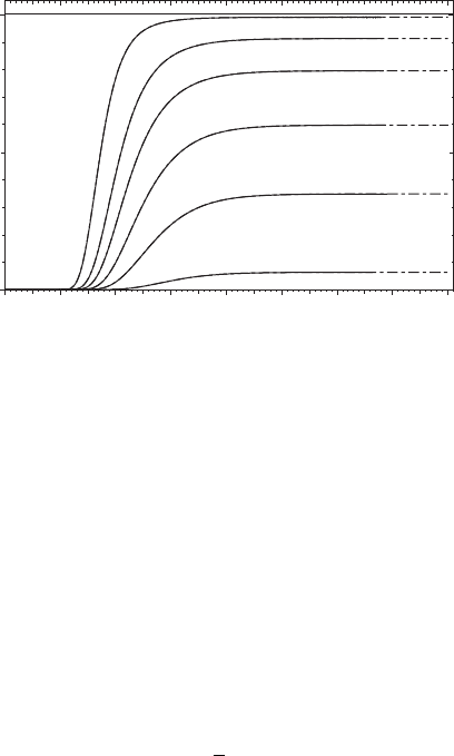
Gaussian like. The transmission probability is computed by integrating the probabil-

ity density ρ over the product region r>7. Figure 21.3 plots several transmission

probabilities as a function of time and energy. The ALE/MLS (Bohmian) results (the

long-short dashed curves) are compared to the results of standard quantum mechani-

cal calculations based on the Crank–Nicholson algorithm (the solid curves). Excellent

agreement between the two sets of results is observed.

Numerical Solution of the Quantum Hydrodynamic Equations 333

0 1020304050607080

0.5

Time (fs)

Probability

0.5 eV

0.8 eV

1.0 eV

1.2 eV

1.4 eV

1.8 eV

FIGURE 21.3 The transmission probability for the one-dimensional wave packet scattering

from an Eckart barrier is plotted as a function of time and energy. The solid curves are computed

using a Crank–Nicholson algorithm and the long-short dashed curves are computed using the

MLS/ALE (Bohmian) approach. The results are essentially identical. For reference a horizontal

line is plotted for unit probability. (Reproduced with permission from Kendrick, B. K., J. Chem.

Phys., 119, 5805, 2003.)

Figure 21.4 plots the 2D potential energy surface for a model collinear chemical

reaction [14]. The potential is given by V = V

(s) +V

(q;s) where the translational

part of the potential is an Eckart function

(s) = V

sech

(as), (21.11)

and the vibrational potential is a local harmonic function

(q;s) =

k(s)q

, (21.12)

where the local force constant is given by k(s) = k

[1 − σ exp(−λ s

)]. The initial

wave packet at time t = 0 is also plotted in Figure 21.4. It is the product of a

ground state harmonic oscillator function for the vibrational motion (q), a Gaussian

wave packet for the translational motion (s), and a phase factor to give it a non-

zero translational velocity. The 2D wave packet was propagated using the MLS/ALE

method including artiﬁcial viscosity [11, 14]. As in the one-dimensional problem

discussed above, the wave packet moves from left to right and tunnels through the

barrier located at s = 0 splitting into transmitted (s>0) and reﬂected (s<0)

components. The probability density associated with the transmitted wave packet

was integrated over all s and q in the product region (s>0) to obtain transmission

probabilities. The transmission probabilities were in excellent agreement with those

computed using the QTM method [14].

The 2D model described above was generalized to higher dimensions (N)by

including additional harmonic oscillator coordinates: q → q

where l = 1, ..., N −1

coupled to the reaction path s. The MLS/ALE method was generalized to this problem