Chattaraj P.K. (Ed.) Quantum Trajectories

Подождите немного. Документ загружается.

354 Quantum Trajectories

As we shall explain below, both disadvantages lead to serious problems when

implementing Wyatt’s idea. However, with little more effort one can establish ﬁtting

algorithms for which both disadvantages appear only in a mild way:

• One idea is to ﬁt a polynomial to the data points (x

, f (x

))

1≤i≤n

such that

it fulﬁlls the following two conditions: First, it goes through the relevant

points where we want to evaluate the derivatives of the function and its

two next neighbors. Second, it gives the best ﬁt in the least squares sense

for all remaining data points. Therefore, one needs to choose a polynomial

degree (m − 1) with 3 <m<n. The advantage hereby is that although

one reproduces the most relevant points the resulting ﬁtting polynomials are

comparably smooth.

• Another idea is to use ﬁtting polynomials with a degree (m −1) with m>n.

This way the ﬁtting polynomial is underdetermined. Among all the polyno-

mials of degree (m −1) which go through all the n data points one chooses

the one with least oscillations as ﬁtting polynomial. The oscillations could

be measured by the largest derivative at all data points.

We shall refer to such ﬁtting methods as “hybrid ﬁtting methods.” Let us point out how

the different ﬁtting methods react to the numerical problems stated in Section 22.2.

When the Grid Point Trajectories Approach Each Other. Let us ﬁrst explain

why least squares ﬁtting is inappropriate in cases of grid point trajectories which

approach each other. Although the algorithm of least squares ﬁtting is well known

for its tendency to stabilize numerical simulations by averaging out numerical errors,

exactly this averaging is responsible for not keeping the grid points on their Bohmian

trajectories in such cases, and thus it is incapable of preventing grid points from

crossing: recall the role of the quantum potential discussed above, cf. Figure 22.1,

and the importance of reproducing the microscopic structure of the wavefunction

during numerical ﬁtting. It is absolutely vital for a numerical simulation to implement

a ﬁtting algorithm that reconstructs not only R, respectively S, in an accurate way

but also its second derivative. The tendency of the least squares ﬁtting algorithm

is to average out those aforementioned small bumps in R, respectively S. As the

simulation is then blind to recognize these bumps in the wavefunction, it is incapable

of recognizing grid points moving toward each other. Grid point trajectory crossings

become unavoidable, and the motion of the grid points is no longer Bohmian.

Note that since the averaging occurs on a microscopic scale, situations in which

grid points move only very slowly or generically do not move toward each other (for

example a free Gaussian wave packet or one approaching a potential creating only

soft reﬂections) are often numerically doable with least squares ﬁtting. On the other

hand numerical simulations with least squares ﬁtting in general situations like the one

we shall discuss in the numerical example below are bound to break down as soon as

two grid points get too close to each other.

A good numerical method must therefore take note of the small bumps and must

prevent their increase. Such a numerical method is provided by polynomial ﬁtting,

since there the polynomials go through all grid points. For this reason polynomial

Bohmian Grids and the Numerics of Schrödinger Evolutions 355

ﬁtting recognizes the bumps of R and S, and hence, the resulting quantum potential

recognizes the approaching grid points. Now recall the physics of the Bohmian time

evolution which, as we have stressed in the introduction, prevents conﬁguration space

trajectories from crossing each other. Therefore, one can expect this method to be self-

correcting and hence stabilizing. For a comparison of polynomial and least squares

ﬁtting see Figure 22.3.

When the Wavefunction Develops Nodes. As described above the problem of

approaching grid point trajectories appears in particular at nodes of the wavefunc-

tion. At nodes R is very small and all effects of the quantum potential Equation 22.9

are ampliﬁed. Averaging out the derivatives on the length scale of grid points may

lead to crossing of grid point trajectories, i.e., the simulated grid point trajectories

may behave unphysically. On the other hand, also exaggeratedly large derivatives

coming from possible highly oscillating polynomials (as, for example, produced by

polynomial ﬁtting) are ampliﬁed. Our later numerical example shows that the former

problem is more severe than the latter. Nevertheless, choosing another ﬁtting method

(we expect the hybrid ﬁtting methods to work very well in general situations) will

give even better results than polynomial ﬁtting.

Note, however, that by equivariance in the vicinity of the nodes of the wavefunction

one expects only a few grid points that may behave badly.

At the Boundary of the Grid. It has to be remarked that polynomial ﬁtting creates a

more severe problem at the boundary of the supporting grid than least squares ﬁtting.

This problem is of a conceptual kind since at the boundary there is a generic lack of

knowledge of how the derivatives of R or S behave, see Figure 22.2.

At the boundary the good property of polynomial ﬁtting, namely to recognize all

small bumps, works against Bohmian grid techniques. On the contrary, least squares

ﬁtting simply averages these small numerical errors out—see the lower right plot in

Figure 22.2. The conceptual boundary problem, however, remains and will show up

eventually also with least squares ﬁtting. Also here we expect better results from the

above mentioned hybrid ﬁtting methods.

Using Equivariance for Stabilization. As discussed in the Introduction, if the grid

points are distributed according to |ψ

, they will remain so for all times. The advan-

tage in this is that now the system is over-determined and the actual density of grid

points must coincide with R

for all times. This could be used as an on the ﬂy check

whether the grid points behave like Bohmian trajectories or not. If not, the numerical

integration does not give a good approximation to the solution of Equations 22.5

through 22.7. It could also be considered to stabilize the numerical simulation with a

feedback mechanism balancing R

and the distribution of the grid points which may

correct numerical errors of one or the other during a running simulation.

22.4 A NUMERICAL EXAMPLE IN MATLAB



The simple numerical example given in this section illustrates the increased numerical

stability when polynomial ﬁtting instead of least squares ﬁtting (least squares ﬁtting

356 Quantum Trajectories

should only be used to ease the boundary problem). This example, however, is clearly

not the optimal method; it is rather meant to support our arguments given so far and can

easily be improved, e.g., using hybrid ﬁtting methods. We shall consider a numerical

example in one dimension with one particle. Therefore, in what follows N = 1 and the

n trajectories are the possible conﬁguration space trajectories (used as a co-moving

grid) of this one particle. We remark, as mentioned earlier, that Gaussian wave packets

are unﬁt for probing the quality of the numerical simulations, because all grid point

will be moving apart from each other and no crossing has to be feared. Therefore, we

take as initial conditions two superposed free Gaussian wave packets with a small

displacement together with a velocity ﬁeld identically zero and focus our attention

on the region where their tails meet, i.e., where the Bohmian trajectories will move

toward each other according to the spreading of the wave packets, see Figure 22.4.

The physical units given in the ﬁgures and the following discussion refer to a wave

packet on a length scale of 1Å = 10

−10

m and a Bohmian particle with the mass of

an electron.

The numerical simulation is implemented as in Ref. [6] with minor changes. It is

written in MATLAB



using IEEE Standard 754 double precision. The source code

can be found in [7]. In order to ease the boundary problem we use a very strong least

squares ﬁtting at the boundary. Note that this only eases the boundary problem and

is by no means a proper cure. In between the boundary, however, the number of data

points for the ﬁtting algorithm and the degree of the ﬁtting polynomial can be chosen

in each run. In this way it is possible to have either polynomial ﬁtting or least squares

ﬁtting in between the boundary. The simulation is run twice: ﬁrst with the polynomial

ﬁtting and then with the least squares ﬁtting algorithm in between the boundaries.

We take seven basis functions for the ﬁtting polynomial in both cases. Note that the

choice should at least be greater or equal to four in order to have enough information

about the third derivative of the ﬁtting polynomial. In the ﬁrst run with polynomial

ﬁtting the number of grid points used for ﬁtting is seven and in the second run for

the least squares ﬁtting we choose nine, which induces a mild least squares behav-

ior. For the numerical integration we have used a time step of 10

−2

fs with a total

0.2

–5

Velocity field (10

m/s)

0.15

0.05

–10 –5 0 5

Position (10

–10

|ψ|

–10

×10

–3

t = 0.02 fst = 0

Analytic |ψ|

Grid points

Analytic velocity field

Grid points

–5 0 5

Position (10

–10

(b)(a)

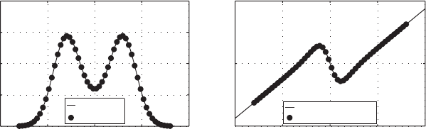
FIGURE 22.4 Left: Initial wavefunction at time zero. Right: Its velocity ﬁeld after a very

short time.

Bohmian Grids and the Numerics of Schrödinger Evolutions 357

0.14

0.13

0.11

0.1

–1.5 –1 –0.5 0 0.5 1 1.5

Position (10

–10

–1.5 –1 –0.5 0 0.5 1 1.5

Position (10

–10

–30 –20 –10 0 10 20 30

Position (10

–10

–30 –20 –10 0 10 20 30

Position (10

–10

(b)

(a)

(d)

(c)

t = 15 fs

t = 3.8 fs

t = 15 fs

t = 3.8 fs

Analytic |ψ|

Fitting polynomials

Grid points

Analytic |ψ|

Fitting polynomials

Grid points

Analytic velocity field

Fitting polynomials

Grid points

Analytic velocity field

Fitting polynomials

Grid points

|ψ|

0.3

0.2

–0.2

Velocity (10

m/s)

–1

–2

Velocity (10

m/s)

0.1

0.05

|ψ|

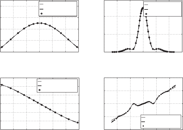
FIGURE 22.5 Simulated |ψ|

together with the velocity ﬁeld at times t = 3.8 fs and t = 15 fs

using polynomial ﬁtting in between the boundary. Left: the center part of the wavefunction

where grid points move toward each other. Right: the whole wavefunction at a later time. The

grid points have all turned and move apart from each other. The kinks at ±20 · 10

−15

min

the velocity ﬁeld in the lower right plot are due to the transition from least squares ﬁtting at

the boundary to polynomial ﬁtting in between the boundary (see paragraph: The Boundary

Problem in Section 22.3).

number of 51 grid points supporting the initial wavefunction. The grid points have

not been |ψ

distributed because in order to see only the differences between least

squares ﬁtting and polynomial ﬁtting the distribution of the grid points does not matter

too much.

Results. The ﬁrst run with polynomial ﬁtting yields accurate results and does not

allow for trajectory crossing way beyond 5000 integration steps, i.e., 50 fs, see Fig-

ures 22.5 and 22.6. The second run with least squares ﬁtting reports a crossing of

trajectories already after 430 integration steps, i.e., 4.3 fs, and aborts, see Figures 22.7

and 22.8. The numerical instability can already be observed earlier, see the left-hand

side of Figure 22.7. An adjustment of the time step of the numerical integration does

not lead to better results in the second run. The crossing of the trajectories of course

occurs exactly in the region were the grid points move fastest toward each other.

Referring to the discussion before, the small bumps in R created by the increase of

the grid point density in this region are not seen by the least squares algorithm and

358 Quantum Trajectories

0.12

0.1

0.08

0.04

0.02

010203040

Time (fs)

Error during simulation Grid point trajectories

(b)(a)

50 60 –10 –5 0 5 10

Position (10

–15

error

Time (fs)

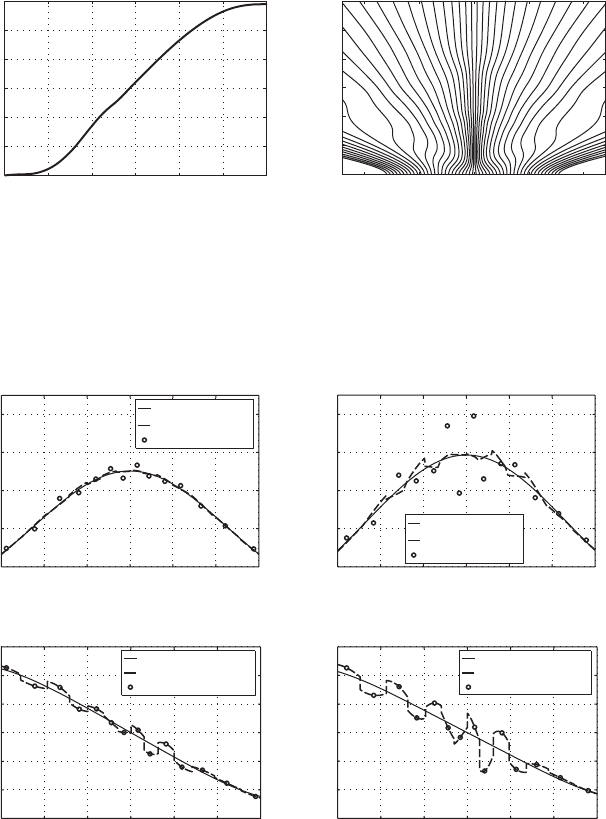
FIGURE 22.6 Both plots belong to the simulation using polynomial ﬁtting in between the

boundary. Left: L

distance between the simulated wavefunction and the analytic solution of

the Schrödinger equation. Right: a plot of the trajectories of the grid points. Note how some

trajectories initially move toward each other, decelerate, and ﬁnally move apart.

0.14

0.13

0.11

0.1

–1.5 –1 –0.5

|ψ|

0.3

0.2

–0.2

Velocity (10

m/s)

0.14

0.13

0.11

0.1

|ψ|

0.3

0.2

–0.2

Velocity (10

m/s)

0 0.5 1 1.5

Position (10

–10

–1.5 –1 –0.5 0 0.5 1 1.5

Position (10

–10

(b)(a)

(d)

(c)

–1.5 –1 –0.5 0 0.5 1 1.5

Position (10

–10

–1.5 –1 –0.5 0 0.5 1 1.5

Position (10

–10

t = 3.8 fs

Analytic |ψ|

Fitting polynomials

Grid points

Analytic |ψ|

Fitting polynomials

Analytic velocity field

Fitting polynomials

Grid points

Analytic velocity field

Fitting polynomials

Grid points

t = 3.8 fs t = 4 fs

t = 4 fs

FIGURE 22.7 Left: same as left-hand side of Figure 22.5 but this time using least squares

ﬁtting throughout. Right: a short time later. Note in the upper left plot, the ﬁtting polynomials

of least squares ﬁtting fail to recognize the relatively big ordinate change of the grid points. So

the grid points moving toward each other are not decelerated by the quantum potential. Finally

after t = 4.3 fs a crossing of the trajectory occurs.

Bohmian Grids and the Numerics of Schrödinger Evolutions 359

Error during simulation

0.12

0.1

0.04

0.02

01 2345

–10 –5 0 5 10

Position (10

–10

Grid point trajectories(b)(a)

Time (fs)

error

Time (fs)

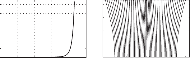
FIGURE 22.8 Both plots belong to the simulation using least squares ﬁtting throughout. Left:

distance between the simulated wavefunction and the analytic solution of the Schrödinger

equation. Right: a plot of the trajectories of the grid points. Note by comparison with right-hand

side of Figure 22.6 the failure of least squares ﬁtting to recognize grid point trajectories moving

toward each other until they ﬁnally cross and the numerical simulation aborts.

thus are not seen by the numerical integration of Equations 22.5 through 22.7, com-

pare Figures 22.5 and 22.7. The approaching grid points are not decelerated by the

quantum potential and ﬁnally cross each other, see Figure 22.7, while in the ﬁrst run

they begin to decelerate and turn to the opposite direction during the time between

3 fs and 5 fs, see Figure 22.5. To visualize how the two algorithms “see” R

and the

velocity ﬁeld during numerical integration these entities have been plotted in Fig-

ures 22.5 and 22.7 by merging all ﬁtting polynomials in the neighborhood of every

grid point together (from halfway to the left neighboring grid point to halfway to the

right neighboring grid point). In Figure 22.7 one clearly observes the failure of the

least squares ﬁtting algorithm to see the small bumps in R.

Note that in some special situations in which the time step of the numerical inte-

gration is chosen to be large, polynomial ﬁtting may lead to trajectory crossing as

well. This may happen when the number of time steps in which the simulation has to

decelerate two fast approaching grid points is not sufﬁcient. This effect is entirely due

to the fact that numerical integration coarse-grains the time. The choice of a smaller

time step for the simulation will always cure the problem as long as other numerical

errors do not accumulate too much.

The relevant measure of quality of the numerical simulation is naturally the L

distance between the simulated wavefunction Re

and the analytic solution of the

Schrödinger equation ψ

, i.e.,





dx |ψ

(x) − R(x, t)e

iS(x,t)



1/2

, and is spelled out

on the left-hand side of Figures 22.6 and 22.8 for both runs.

BIBLIOGRAPHY

1. S. Goldstein. Bohmian Mechanics. Contribution to Stanford Encyclopedia of Philosophy,

ed. by E.N. Zalta, 2001. http://plato.stanford.edu/entries/qm-bohm/

2. D. Dürr and S. Teufel Bohmian Mechanics. Springer, Berlin, 2009.

360 Quantum Trajectories

3. D. Dürr, S. Goldstein, and N. Zanghì. Quantum Equilibrium and the Origin of Absolute

Uncertainty. J. Statist. Phys., 67:843–907, 1992.

4. S. Teufel and R. Tumulka. Simple Proof for Global Existence of Bohmian Trajectories.

Commun. Math. Phys., (258):349–365, 2005.

5. D. Dürr, S. Goldstein, and N. Zanghì. Quantum Equilibrium and the Role of Operators as

Observables in Quantum Theory. J. Statist. Phys., 116:959–1055, 2004.

6. R.E. Wyatt. Quantum Dynamics with Trajectories. Springer, New York, 2005.

7. D.-A. Deckert, D. Dürr, and P. Pickl. Quantum Dynamics with Bohmian Trajectories.

arXiv:quant-ph/0701190, 2007.

Approximate Quantum

Trajectory Dynamics

in Imaginary and Real

Time; Calculation

of Reaction Rate Constants

Sophya Garashchuk

CONTENTS

23.1 Introduction.................................................................................................361

23.2 Calculation of N (E) Within the Flux Operator Formalism With

Approximate Quantum Trajectories............................................................363

23.2.1 Real-Time Variational Approximate Quantum Potential ..............364

23.2.2 Wavepacket Evolution and Computation of Correlation

Functions in the Mixed Coordinate/Polar Representation............366

23.2.3 Numerical Illustration ...................................................................366

23.3 Trajectory Dynamics in Imaginary Time With the Momentum-

Dependent Quantum Potential....................................................................368

23.3.1 Equations of Motion .....................................................................368

23.3.2 Approximate Implementation and Excited States.........................369

23.3.3 Calculation of the Energy Levels..................................................371

23.4 Computation of Reaction Rates From the Imaginary and Real-Time

Quantum Trajectory Dynamics...................................................................373

23.5 Summary.....................................................................................................375

Acknowledgments..................................................................................................377

Bibliography ..........................................................................................................377

23.1 INTRODUCTION

In this chapter we formulate quantum trajectory dynamics in imaginary time which

seamlessly connects to Bohmian dynamics in real time. Approximate determination

of the quantum potential and mixed representation of wavefunctions with nodes make

this trajectory approach stable and scalable to high dimensions, while including the

361

362 Quantum Trajectories

leading quantum effects into wavefunction evolution. Reaction probabilities, energy

eigenstates and reaction rate constants can be obtained by propagating an ensemble

of quantum trajectories in real and/or imaginary time.

Most of the quantum-mechanical (QM) theoretical studies of thermal reaction rate

constants, k(T ), and cumulative reaction probabilities, N (E), are based on the trace

expressions [1], that involve evolution operators—the Hamiltonian operator in real

time and the Boltzmann operator in inverse temperature, equivalent to imaginary

time—and the symmetrized ﬂux operator,

F =

[ˆp, δ(x − x

)]. (23.1)

The function δ(x −x

) is the Dirac δ-function; x is the reaction coordinate, m is the

reduced mass conjugate to x, and x

is the location of the surface dividing reactants

and products. In atomic units the cumulative reaction probability is

N(E) = 2π

Tr[

F δ(E −

H )

F δ(E −

H )]. (23.2)

The thermal reaction rate constant,

k(T ) = Q

−1

(T )



∞

(t)dt, (23.3)

can be found from the ﬂux–ﬂux correlation function C

(t),

(t) = Tr[e

−β

H /2

−β

H /2

−ı

]. (23.4)

In the above equations T labels temperature, Q(T ) is the reactant partition function,

and β = (k

T )

−1

is the thermal evolution variable, where k

is the Boltzmann con-

stant. The real time is labeled t; x

is set to zero for both dividing surfaces. While N (E)

is a more general quantity from which the reaction rate constants can be computed

for any temperature,

2πk(T )Q(T ) =



∞

−∞

−βE

N(E)dE, (23.5)

Equations 23.3 and 23.4 can be better suited for numerical evaluation due to the

damping effect of the Boltzmann operator, exp(−β

H ), suppressing wavefunction

oscillations.

In general, to describe the dynamics of several (more than four) nuclei, approximate

wavefunction evolution methods are needed, because the conventional grid- or basis-

based QM methods [2] scale exponentially with the system size. The trajectory-based

propagation techniques, such as those of Refs [3–8], combining intuitiveness and

low cost of classical mechanics with a description of the leading quantum effects

on dynamics of nuclei provide appealing alternatives. Several recent approaches

[9–14] are based on the de Broglie–Bohm formulation of the Schrödinger equation,

Approximate Quantum Trajectory Dynamics in Imaginary and Real Time 363

where the wavefunction is represented by the quantum trajectories propagated

with approximations to its derivatives. We develop dynamics with globally deter-

mined approximations to the quantum potential: In Section 23.2 we show how to

compute the cumulative reaction probability Equation 23.2 by propagating Gaussian-

based eigensolutions of the ﬂux operator [15] using the variational Approximate

Quantum Potential (AQP) [9] and the mixed wavefunction representation [16,17]; in

Section 23.3 we describe the imaginary-time quantum trajectory dynamics with the

momentum-dependent quantum potential (MDQP) [18] suitable for computation of

low-lying energy eigenstates; in Section 23.4 we combine real and imaginary-time

dynamics to compute reaction rates from Equation 23.3 to Equation 23.4. For imple-

mentations that are cheap and scalable to many dimensions, the MDQP is determined

by ﬁtting the trajectory momenta in a small basis, also used to evolve wavefunctions

with nodes.

All derivations are given in one Cartesian dimension, x = (−∞, ∞), in atomic

units. ∇ denotes differentiation with respect to x for compactness. Planck’s constant is

explicitly included in several places to emphasize the -dependence of the quantum

potential. One-dimensional numerical illustrations are given for anharmonic wells

and for the Eckart barrier modeling the transition state of H

23.2 CALCULATION OF N(E ) WITHIN THE FLUX

OPERATOR FORMALISM WITH APPROXIMATE

QUANTUM TRAJECTORIES

As ﬁrst observed numerically [19], in a ﬁnite basis the singular operator

F given by

Equation 23.1 has just two nonzero eigenvalues, which enabled efﬁcient QM calcula-

tions of N(E) for tetratomic systems using the transition state wavepackets [20,21].

The two eigenvalues are negatives of each other and the corresponding eigenvectors

are complex conjugates,

F |φ

=±λ|φ

, |φ



∗

=|φ

−

. (23.6)

Substituting the spectral representation of

F and the integral expression of δ(E −

H ),

2πδ(E −

H ) =



∞

−∞

−ı

ıEt

dt,

into Equation 23.2, N(E) can be written through the wavepacket correlation func-

tions C

=φ

(0)|φ

−

(t), (23.7)

N(E) = λ





∞

−∞

ıEt

−



∞

−∞

−

ıEt



. (23.8)

The eigensolutions of

F in a ﬁnite basis, derived analytically by Seideman and Miller

[22], can be expressed in terms of the Dirac δ-function [15],

δ(x)

√

2δ|δ

∓

ı∇δ(x)

√

2∇δ|∇δ

, λ =

√

δ|δ∇δ|∇δ

. (23.9)