Chattaraj P.K. (Ed.) Quantum Trajectories
Подождите немного. Документ загружается.

104 Quantum Trajectories
0
0.2
0.4
0.6
0.8
1
0 1000 2000 3000 4000
Tunneling probability
Time (a.u.)
C1
C2
C3
Q1
Q2
Q3
E1
E2
E3
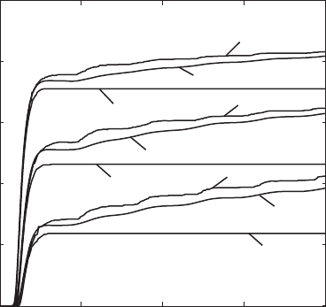
FIGURE 7.2 Time-dependent tunneling probabilities. Three initial wave packets or ensem-
bles are considered, and the results of the entangled trajectory molecular dynamics simulations
(E) are compared with purely classical (C) and exact quantum (Q) calculations. See the text
for details.
labeled C, Q, and E indicate classical, quantum, and entangled trajectory ensemble
results, respectively. Case 1 corresponds to a mean energy E
o
=ψ|
ˆ
H |ψ#0.75V
‡
.
For case 2, E
o
# 1.25 V
‡
, while for case 3, E
o
# 2.0 V
‡
. Increasing the mean
energy increases the short time transfer across the barrier, both classically and quan-
tum mechanically. The classical reaction, however, ceases immediately after the first
sharp rise, as the trajectories in the ensemble with energy below the barrier initially
are trapped there for all time. The quantum wave packet, however, continues to escape
from the metastable well by tunneling, and the reaction probability continues to grow
slowly with time following the initial classical-like rise. This growth is modulated
by the oscillations of the wave packet in the potential well. The entangled trajec-
tory calculation tracks the exact quantum results quite well. Although these results
slightly overestimate the exact instantaneous probability, the qualitative dynamics
are described quite satisfactorily. In particular, the purely nonclassical longer time
growth of the reaction probability is correctly described.
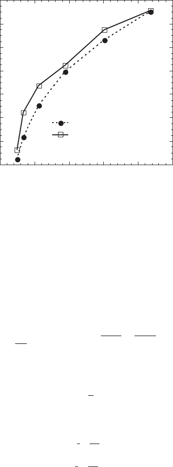
In Figure 7.3, we examine the agreement between quantum and entangled trajec-
tory predictions of the non-classical tunneling dynamics in more detail. The decay of
the survival probability 1−P (t) at times longer than the initial rapid classical decay is
fit to an exponential exp(−kt) and the tunneling rate constant k thus defined is plotted
in the figure as a function of mean wave packet energy. The overall correspondence
is very good, especially considering that a nonzero k is a quantity that results solely
from the non-classical tunneling of the particle through the barrier.
Quantum Trajectories in Phase Space 105
0.0
0.2
0.4
0.6
0.8
1.0
1.2
1.4
0.00 0.01 0.02 0.03 0.04 0.05
Exact quantum
Entangled trajectories
Energy (a.u.)
Rate (10
–5
a.u.)
FIGURE 7.3 Tunneling rate as a function of initial mean wave packet energy, entangled tra-
jectory molecular dynamics and exact quantum results.
7.5 HUSIMI REPRESENTATION
The above method employs local smoothing implicitly to formulate an entangled
trajectory method in the Wigner representation. We now formalize this idea by a
generalization of the approach that is based on a rigorous positive phase space repre-
sentation of quantum mechanics: the Husimi representation [13].
The Husimi distribution is a locally smoothed Wigner function:
ρ
H
(q, p) =
1
π
∞
−∞
ρ
W
(q
, p
)e
−
(q−q
)
2
2σ
2
q
e
−
(p−p
)
2
2σ
2
p
dq
dp
(7.36)
where the smoothing is over a minimum uncertainty phase space Gaussian, satisfying
σ
q
σ
p
=
2
. (7.37)
The smoothing can be represented using smoothing operators
ˆ
Q and
ˆ
P :
ˆ
Q = e
1
2
σ
2
q
∂
2
∂q
2
(7.38)
ˆ
P = e
1
2
σ
2
p
∂
2
∂p
2
. (7.39)
The Husimi can then be written as a smoothed Wigner function as:
ρ
H
(q, p) =
ˆ
Q
ˆ
P ρ
W
(q, p). (7.40)

106 Quantum Trajectories
This is related to the interesting identity:
e
−a(x−x
)
2
= e
1
4a
∂
2
∂x
2
δ(x −x
). (7.41)
We can consider the inverse unsmoothing operators
ˆ
Q
−1
and
ˆ
P
−1
:
ˆ
Q
−1
= e
−
1
2
σ
2
q
∂
2
∂q
2
(7.42)
ˆ
P
−1
= e
−
1
2
σ
2
p
∂
2
∂p
2
(7.43)
so that the Wigner function can be written (at least formally) as an “unsmoothed”
Husimi:
ρ
W
(q, p) =
ˆ
Q
−1
ˆ
P
−1
ρ
H
(q, p). (7.44)
We can then derive an equation of motion for the Husimi distribution
∂ρ
H
∂t
=−
1
m
ˆ
Pp
ˆ
P
−1
∂ρ
H
∂q
+
∞
−∞
ˆ
QJ (q, η)
ˆ
Q
−1
ρ
H
(q, p +η, t) dξ. (7.45)
Note that there are no approximations; the Husimi representation provides an exact
alternative description of quantum dynamics.
In the Husimi representation, powers of the coordinates and momenta become
differential operators:
ˆ
Qq
ˆ
Q
−1
= q + σ
2
q
∂
∂q
(7.46)
ˆ
Pp
ˆ
P
−1
= p + σ
2
p
∂
∂p
(7.47)
ˆ
Qq
2
ˆ
Q
−1
= q
2
+ σ
2
q
+ 2σ
2
q
q
∂
∂q
+ σ
4
q
∂
2
∂q
2
. (7.48)
The Husimi equation of motion for the cubic system can then be written:
∂ρ
H
∂t
=−
1
m
ˆ
Pp
ˆ
P
−1
∂ρ
H
∂q
+ (mω
2
o
ˆ
Qq
ˆ
Q
−1
− b
ˆ
Qq
2
ˆ
Q
−1
)
∂ρ
H
∂p
+
2
b
12
∂
3
ρ
H
∂p
3
(7.49)
where
ˆ
Qq
ˆ
Q
−1
= q + σ
2
q
∂
∂q
(7.50)
ˆ
Pp
ˆ
P
−1
= p + σ
2
p
∂
∂p
(7.51)
ˆ
Qq
2
ˆ
Q
−1
= q
2
+ σ
2
q
+ 2σ
2
q
q
∂
∂q
+ σ
4
q
∂
2
∂q
2
. (7.52)

Quantum Trajectories in Phase Space 107
Continuity conditions can be applied in the Husimi representation, which are now
rigorously justified for a positive probability distribution:
∂ρ
H
∂t
+
!
∇·
!
j
H
= 0. (7.53)
This yields an expression for the divergence of the phase space current,
!
∇·
!
j
H
=
∂
∂q
p
m
ρ
H
+
∂
∂p
− V
(q)ρ
H
+
b
2mω
o
ρ
H
+
bq
mω
o
∂ρ
H
∂q
+
2
b
4m
2
ω
2
o
∂
2
ρ
H
∂q
2
−
2
b
12
∂
2
ρ
H
∂p
2
. (7.54)
The phase space vector field can then be written as
˙q =
p
m
(7.55)
˙p =−V
(q) +
b
2mω
o
+
bq
mω
o
1
ρ
H
∂ρ
H
∂q
+
2
b
4m
2
ω
2
o
1
ρ
H
∂
2
ρ
H
∂q
2
−
2
b
12
1
ρ
H
∂
2
ρ
H
∂p
2
.
(7.56)
The quantum force now contains additional terms not present in the Wigner repre-
sentation quantum force. It is interesting to note that, because of the smoothing, the
motion of a free particle is nonclassical in the Husimi representation,
∂ρ
H
∂t
=−
1
m
ˆ
Pp
ˆ
P
−1
∂ρ
H
∂q
(7.57)
or
∂ρ
H
∂t
=−
1
m
p
∂ρ
H
∂q
−
σ
2
p
m
∂
2
ρ
H
∂q∂p
. (7.58)
The extra terms are due to noncommutativity of classical time evolution and smooth-
ing. (For a harmonic oscillator, the cross-terms resulting from the kinetic energy and
potential energy cancel, leading to classical evolution.)
The MD methodology described above can be easily generalized to incorpo-
rate the additional terms in the equations of motion in the Husimi representation.
When implemented, excellent agreement with exact results for model systems is
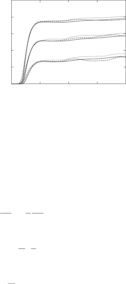
again obtained [13]. In Figure 7.4, results for the cubic system are shown, indicat-
ing the level of agreement between exact quantum results, the Wigner-based method
described above, and the implementation based on the positive Husimi representation.
7.6 INTEGRODIFFERENTIAL EQUATION FORM
The methods above have been based on an expansion of the quantum phase space
density and potential in power series. When using a discrete representation of the den-
sity in terms of a sum of delta functions, Equation 7.12, the estimation of higher order
108 Quantum Trajectories
0
0.2
0.4
0.6
0.8
1
0 500 1000 1500 2000
(a)
(b)
(c)
Tunneling probability
Time (a.u.)
FIGURE 7.4 Tunneling probabilities versus time. Solid lines represent exact results. Fine
dotted lines show results for the entangled trajectory method based on an expansion of the
Wigner function, as described in the text. Dashed lines present results performed in the Husimi
representation. Cases a, b, and c refer to the initial placement of the center of the wave packet
q
0
=−0.2 au, q
0
=−0.3 au, and q
0
=−0.4 au, respectively.
derivatives of ρ
W
from this form is challenging. It is more natural to work directly
with the integrodifferential equation form of the equations of motion, Equation 7.7,
where the nonlocality of quantum mechanics is expressed explicitly as a convolution
without any power series expansion and the discrete representation of ρ
W
can be
employed directly. With this in mind, we return to the Wigner equation of motion in
the integrodifferential form, and try to solve it directly:
∂ρ
W
∂t
=−
p
m
∂ρ
W
∂q
+
∞
−∞
J (q, p − ξ)ρ
W
(q, ξ, t)dξ. (7.59)
We write the divergence of the flux as:
!
∇·
!
j
W
=
∂
∂q
p
m
ρ
W
−
∞
−∞
J (q, ξ − p) ρ
W
(q, ξ, t) dξ. (7.60)
The momentum component of the flux divergence is then:
∂
∂p
j
W ,p
=−
∞
−∞
J (q, ξ − p) ρ
W
(q, ξ, t) dξ. (7.61)
Integrating, we obtain
j
W ,p
=−
∞
−∞
Θ(q, ξ − p) ρ
W
(q, ξ, t) dξ, (7.62)

Quantum Trajectories in Phase Space 109
where
Θ(q, ξ − p) =
p
−∞
J (q, ξ − z) dz. (7.63)
This can be written explicitly in terms of the potential V (q):
Θ(q, ξ − p) =
1
2π
∞
−∞
3
V
q +
y
2
− V
q −
y
2
4
e
−i(ξ−p)y/
y
dy. (7.64)
The quantum trajectory equations of motion then become
˙q =
p
m
(7.65)
˙p =−
1
ρ
W
(q, p)
Θ(q, p −ξ)ρ
W
(q, ξ) dξ. (7.66)
To proceed numerically, we write the Wigner function as a superposition of
Gaussians:
ρ
W
(q, p, t) =
1
N
N
j=1
φ(q − q
j
(t), p − p
j
(t)), (7.67)
where
φ(q, p) =
1
2ψ
q
σ
p
exp
−
q
2
2σ
2
q
−
p
2
2σ
2
p
. (7.68)
After some algebra, we find
˙p(q, p) =−
N
j=1
φ
q
(q − q
j
)Λ(q − q
j
, p −p
j
)
N
j=1
φ
q
(q − q
j
)φ
p
(q − q
j
)
(7.69)
where
Λ(q − q
j
, p −p
j
) =
V (q +z/2) −V (q − z/2)
z
exp
i
(p −p
j
)z
−
σ
2
p
z
2
2
2
dz.
(7.70)
This can be evaluated numerically for a given potential V (q).
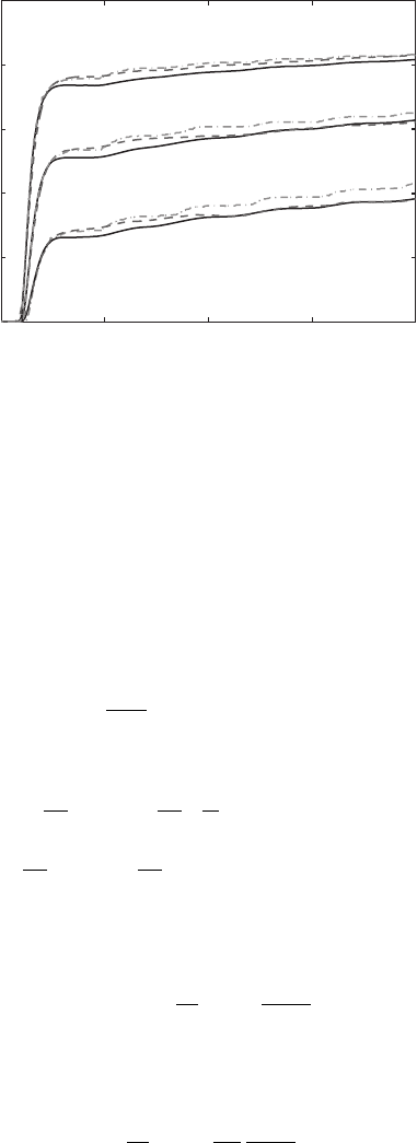
The results of this method are shown in Figure 7.5, and compared with both the
exact quantum results and the Wigner method based on an expansion in , described
above. The integrodifferential equation method yields better agreement with exact
results, particularly at longer times. It should be noted that this implementation
incorporates the purely classical part of the equations of motion in the kernel Λ(q, p),
giving a classical mechanics where the potential V (q), rather than the force −V
(q),
appears in the equations of motion.
110 Quantum Trajectories
0 1000 2000 3000 4000
0
0.2
0.4
0.6
0.8
1
Time (a.u.)
Tunneling probability
(c)
(b)
(a)
FIGURE 7.5 Time-dependent reaction probabilities for the cubic potential system with three
different initial energies E
0
= 0.75 V
0
(a), E
0
= 1.25 V
0
(b), and E
0
= 2.0 V
0
(c). Solid,
dashed, and dash-dotted lines represent the results of an exact quantum calculation, entangled
trajectory simulations using the integrodifferential equation formulation, Equation 7.69, and
the results using the expansion in powers of , respectively.
7.7 GAUGE FREEDOM IN PHASE SPACE
We now briefly consider a gauge-like freedom in the definition of the vector field
that phase space trajectories follow in our approach. We can express our continuity
equation
∂ρ
W
∂t
+ ∇ ·j
W
= 0 (7.71)
in terms of the components as
∂
∂q
( ˙qρ
W
) =
∂
∂q
p
m
ρ
W
+ θ
q
ρ
W
∂
∂p
( ˙pρ
W
) =
∂
∂p
−V
(q)ρ
W
+ θ
p
ρ
W
(7.72)
which defines the “quantum vector field” θ = (θ
q
, θ
p
). We then consider the condition
for the non-classical terms in the equations of motion:
∇·(θρ
W
) =
2
24
V
(q)
∂
3
ρ
W
∂p
3
. (7.73)
There is freedom in the solution of this differential equation for the vector θ. With the
choice θ
q
= 0, Equation 7.73 can be integrated to yield
θ
p
=
2
24
V
(q)
1
ρ
W
∂
2
ρ
W
∂p
2
. (7.74)

Quantum Trajectories in Phase Space 111
This recovers the basis of the method described in this chapter [9–13]. Other choices
are possible, however. For instance, we can choose θ
p
= 0, which then yields
θ
q
=
2
24
1
ρ
W
q
V
(q
)
∂
3
ρ
W
(q
, p)
∂p
3
dq
. (7.75)
This defines an alternative (and untested) quantum trajectory method. Many other
divisions of the quantum vector field between its q and p components are possible,
which all lead to the same quantum Liouville equation. In general, we can take a
quantum trajectory method with non-classical term θ and add to the vector field any
additional term ψ such that θ → θ +ψ and obtain an alternative quantum trajectory
method, as long as the condition ∇·ψ = 0 is satisfied. This gauge-like freedom in
the definition of quantum trajectories highlights their role simply as mathematical
elements of the overall numerical method employed to represent the unified state of
the system ρ
W
, rather than as realistic descriptions of the actual paths of quantum
particles—in other words, as hidden variables [14,17–19].
7.8 DISCUSSION
The entangled trajectory formalism described in this chapter gives a unique but intu-
itively appealing picture of the quantum tunneling process. Rather than portraying
tunneling as a “burrowing” through the barrier, trajectories that successfully sur-
mount the obstacle do so by “borrowing” energy from their fellow ensemble mem-
bers, and then going over the top in a classical-like manner. This energy loan is then
paid back through the nonlocal inter-trajectory interactions, always keeping the mean
energy of the ensemble a constant.
We have described an approach to the simulation of quantum processes using a
generalization of classical MD and ensemble averaging. The general method was
illustrated for the nonclassical phenomenon of quantum tunneling through a potential
barrier. The basis of the method is the Liouville representation of quantum mechanics
and its realization in phase space using the Wigner representation, or its generalization
to strictly positive phase space densities, the Husimi representation. The evolution
of the phase space functions is approximated by representing the distribution by a
collection of trajectories, and then propagating equations of motion for the trajectory
ensemble. In the classical limit, the members of the ensemble evolve independently
under Hamilton’s equations of motion. When quantum effects are included, however,
the resulting quantum trajectories are no longer separable from each other. Rather,
their statistical independence is destroyed by nonclassical interactions that reflect the
nonlocality of quantum mechanics. Their time histories become interdependent and
the evolution of the quantum ensemble must be accomplished by taking this entan-
glement into account.
BIBLIOGRAPHY
1. C. Cohen-Tannoudji, B. Diu, and F. Laloe, Quantum Mechanics (John Wiley, New York,
1977).
112 Quantum Trajectories
2. G. C. Schatz and M. A. Ratner, Quantum Mechanics in Chemistry (Prentice Hall, Engle-
wood Cliffs, 1993).
3. M. P. Allen and D. J. Tildesley, Computer Simulation of Liquids (Clarendon Press, Oxford,
1987).
4. H. Goldstein, Classical Mechanics (Addison-Wesley, Reading, MA, 1980), 2nd ed.
5. E. P. Wigner, Phys. Rev. 40, 749 (1932).
6. K. Takahashi, Prog. Theor. Phys. Suppl. 98, 109 (1989).
7. H. W. Lee, Phys. Rep. 259, 147 (1995).
8. S. Mukamel, Principles of Nonlinear Optical Spectroscopy (Oxford University Press,
Oxford, 1995).
9. A. Donoso and C. C. Martens, Phys. Rev. Lett. 87, 223202 (2001).
10. A. Donoso and C. C. Martens, Int. J. Quantum Chem. 87, 1348 (2002).
11. A. Donoso and C. C. Martens, J. Chem. Phys. 116, 10598 (2002).
12. A. Donoso, Y. Zheng, and C. C. Martens, J. Chem. Phys. 119, 5010 (2003).
13. H. López, C. C. Martens, and A. Donoso, J. Chem. Phys. 1125, 154111 (2006).
14. R. Wyatt, Quantum Dynamics with Trajectories: Introduction to Quantum Hydrodynamics
(Springer, New York, 2005).
15. D. A. McQuarrie, Statistical Mechanics (HarperCollins, New York, 1976).
16. R. Kosloff, Ann. Rev. Phys. Chem. 45, 145 (1994).
17. D. Bohm, Phys. Rev. 85, 166 (1952).
18. D. Bohm, Phys. Rev. 85, 180 (1952).
19. P. R. Holland, The Quantum Theory of Motion (Cambridge University Press, Cambridge,
1995).

8
On the Possibility of
Empirically Probing the
Bohmian Model in Terms
of the Testability of
Quantum Arrival/Transit
Time Distribution
Dipankar Home and Alok Kumar Pan
CONTENTS
8.1 Introduction and Motivation ......................................................................... 113
8.2 The Setup ...................................................................................................... 117
8.3 The Testable Probabilities.............................................................................118
8.4 The Evaluation of Π(t) and Π(φ) Using the Bohmian Model......................119
8.5 Subtleties in the Bohmian Calculation of Π(t) and Π(φ).............................124
8.6 Summary and Outlook ..................................................................................126
Appendix A ............................................................................................................127
Acknowledgments..................................................................................................131
Bibliography ..........................................................................................................131
8.1 INTRODUCTION AND MOTIVATION
Born’s interpretation of the squared modulus of a wave function (
|
ψ
|
2
) as the prob-
ability density of finding a particle within a specified region of space is a key ingre-
dient of the standard framework of quantum mechanics, thereby implying that the
standard interpretation of quantum mechanics is inherently epistemological. On the
other hand, the possibility of an alternative interpretation of quantum mechanics
by interpreting
|
ψ
|
2
as the probability density of a particle being actually present
within a specified region was first suggested by de Broglie [1]. Later, Bohm [2–4]
developed the details of such an ontological model of quantum mechanics by using
the notion of an observer-independent spacetime trajectory of an individual particle
113