Chattaraj P.K. (Ed.) Quantum Trajectories

Подождите немного. Документ загружается.

94 Quantum Trajectories

overall motion. This motion is simply the classical motion due to the sum of the

uniform and linear forces; the addition of the uniform force has no other effect on the

state’s time evolution.

6.5 CONCLUSION

The quantum force formulation of Bohmian mechanics offers concepts, tools, and

language that are unavailable in either standard quantum mechanics or in the

Hamilton–Jacobi formulation of Bohmian mechanics. Though these features are

unlikely to render easily soluble those problems that are intractable in standard quan-

tum mechanics, or in the HJ formulation of Bohmian mechanics, the quantum force

formulation remains inherently valuable for the unique methods and insights it makes

available to us.

ACKNOWLEDGMENTS

Michelle McMillan carried out considerable work related to Section 6.4.3. I thank

my friend and colleague, Ralph Baierlein, for critically reading the manuscript, and

Pratim Chattaraj for the opportunity to contribute to this volume, as well as for his

patience and understanding. I also thankAmy Caldwell, for giving me reason to go on.

This work is dedicated to the memory of my wife Katherine, through whom I

learned the meaning of devotion.

BIBLIOGRAPHY

1. Bohm, D., 1952. A suggested interpretation of the quantum theory in terms of hidden

variables, I. Phys. Rev. 85:166–79.

2. Bohm, D., 1952. A suggested interpretation of the quantum theory in terms of hidden

variables, II. Phys. Rev. 85:180–93.

3. Goldstein, H., 1980. Classical Mechanics, 2nd edn. (Reading, MA: Addison-Wesley).

4. Bowman, G., 2006. Quantum-mechanical time evolution and uniform forces. J. Phys. A

39:157–62.

5. Bowman, G., 2002. Bohmian mechanics as a heuristic device: wave packets in the harmonic

oscillator. Am. J. Phys. 70:313–18.

6. Messiah, A., 1964. Quantum Mechanics (Amsterdam: North-Holland).

7. McMillan, M. and Bowman, G., Gaussian wavepacket evolution in time-dependent

quadratic potentials (in preparation).

Quantum Trajectories

in Phase Space

Craig C. Martens, Arnaldo Donoso,

and Yujun Zheng

CONTENTS

7.1 Introduction.....................................................................................................95

7.2 Dynamics in Phase Space ...............................................................................96

7.3 Quantum Trajectories......................................................................................99

7.4 Entangled Trajectory Molecular Dynamics ..................................................101

7.5 Husimi Representation..................................................................................105

7.6 Integrodifferential Equation Form ................................................................107

7.7 Gauge Freedom in Phase Space.................................................................... 110

7.8 Discussion ..................................................................................................... 111

Bibliography .......................................................................................................... 111

7.1 INTRODUCTION

Since the time our prehistoric ancestors ﬁrst portrayed motion by scratching a line in

the dirt with the point of a spear, we have most naturally described dynamics with

trajectories—paths though space parameterized by time. This eventually became for-

malized in the classical mechanics of particles by Newton, Lagrange, Hamilton, and

others. Despite the formidable mathematical sophistication that classical dynamics

can exhibit, the primordial intuition of matter being composed of things that can be

found at a deﬁnite place at a given time remains at its foundation.

Quantum mechanics is the proper theoretical framework for describing the behav-

ior of matter when it is composed of atoms and molecules [1, 2]. The unassailable

successes of quantum mechanics in predicting the properties of matter at this scale

are well-known. Equally well-known are the profound problems underlying the inter-

pretation of the theory. The reconciliation of quantum effects such as the uncertainty

principle, wave–particle duality, wave function collapse, entanglement, and others

with the intrinsic classical perspective we view the world has a long and continuing

history. A central part of this history is the desire to recover a “realistic” description

of particle motion in quantum systems in terms of “hidden variables”—underlying

classical-like paths that satisfy the desire for a description of nature that allow par-

ticles to always be somewhere deﬁnite. Developments along the way, in particular

96 Quantum Trajectories

Bell’s theorem, have gone a long way in excluding hidden variables and enforcing

the need to retain the nonclassical and nonintuitive elements of quantum mechan-

ics. Nonetheless, efforts to understand quantum mechanics and the correspondence

principle continue in corners of physical science and philosophy.

Most applications of theory—whether classical or quantum—to describing phys-

ical systems are made for practical rather than philosophical reasons. This is another

area where classical mechanics often has an advantage over quantum mechanics. In

this chapter we consider the problem of simulating quantum processes in molecular

systems using classical trajectories and ensemble averaging. We mainly focus on the

methodology rather than issues of interpretation.

For simple systems, a direct numerical solution of the time-dependent Schrödinger

equation can be accomplished easily. For complex many-body problems the unfavor-

able scaling of computational cost of standard quantum methods with dimension and

particle number make this approach intractable, and approximate methods must be

employed. A broad range of such approaches have been developed, including mean-

ﬁeld methods, semiclassical and mixed classical–quantum methods, phenomenolog-

ical reduced descriptions, and others.

One surprisingly effective approach in many cases is to simply ignore quantum

effects altogether and use classical mechanics to describe the motion of atoms in

molecular systems. The result is the method called classical molecular dynamics

(MD) [3], a commonly used approach for studying many-particle systems where

high temperatures, large masses, or other factors allow quantum effects in the atomic

motion to be neglected. An MD simulation is performed by solving the appropriate

Hamilton or Newton equations of motion given the forces of interaction and appropri-

ate initial conditions. An individual classical trajectory for a multidimensional prob-

lem is much easier to integrate numerically than the time-dependent wave packet of the

corresponding quantum system. Unless the anecdotal information revealed by a single

trajectory is sufﬁcient, however, signiﬁcant numbers of trajectories—ensembles—

must be employed. A distribution of trajectories evolving in phase space is the most

direct classical analogue of an evolving quantum wave packet, and statistical aver-

ages of dynamical variables over the classical ensemble parallel the corresponding

quantum expectation values of operators.

7.2 DYNAMICS IN PHASE SPACE

The state of a classical system is represented by a probability distribution ρ(q, p, t)

deﬁned in the phase space (q, p) of the system. The evolution of ρ(q, p, t) in phase

space is governed by the classical Liouville equation [4]

∂ρ

∂t

={H , ρ}, (7.1)

where we consider a system with one degree of freedom for simplicity; this can

be easily generalized. The q and p are the canonical coordinate and momentum,

respectively, H (q, p) = p

/2m + V (q) is the system Hamiltonian, where m is the

Quantum Trajectories in Phase Space 97

mass and V (q) is the potential energy function, and {H , ρ} is the Poisson bracket of

H and ρ, deﬁned as

{H , ρ}≡

∂H

∂q

∂ρ

∂p

−

∂ρ

∂q

∂H

∂p

. (7.2)

In classical MD, a solution of the Liouville equation is approximated by generating an

ensemble of N distinct initial conditions q

(0) and p

(0) (k = 1,2, ...,N ) sampled

from the given initial probability distribution ρ(q, p, 0). Phase space trajectories are

then determined by integrating the Hamilton equations,

˙q =

∂H

∂p

(7.3)

˙p =−

∂H

∂q

(7.4)

using the q

(0) and p

(0) as initial data. Then, aside from statistical error due to a

ﬁnite N, ρ(q, p, t) is given by the local phase space density of the evolving trajectories

(t), p

(t)) around the point (q, p). The relation between the evolution of the clas-

sical function ρ(q, p, t) and the trajectory ensemble (q

(t), p

(t)) (k = 1,2, ...,N)

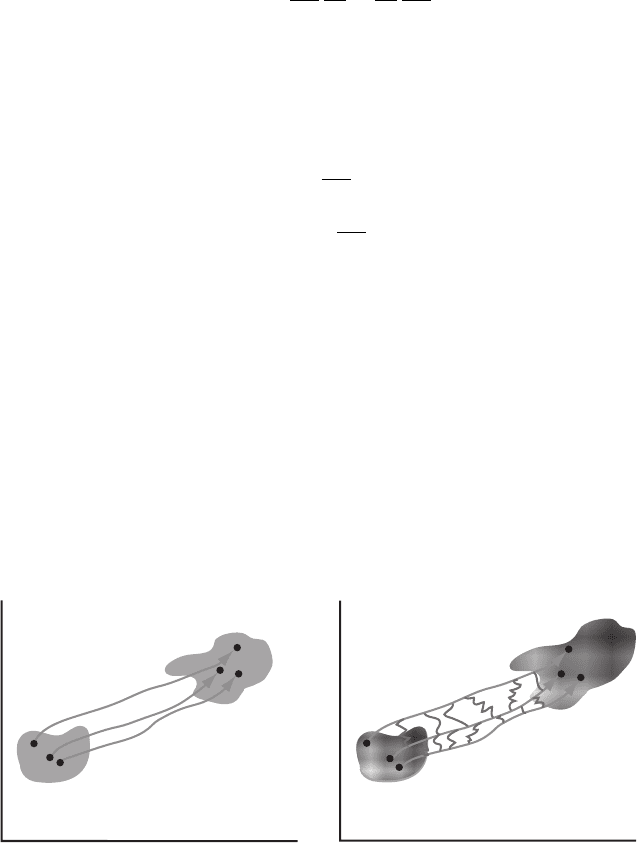
in phase space is illustrated schematically in the left panel of Figure 7.1.

Our goal is to describe quantum mechanics from a similar phase space trajectory

ensemble perspective. To accomplish this, we adopt a phase space representation

of quantum mechanics—the Wigner representation [5–8]. The quantum state of the

system that was described using classical mechanics above is now represented by

the wave function ψ(q, t), which is a solution of the time-dependent Schrödinger

equation [1]. An equivalent phase space description is given in terms of the Wigner

ρ(q,p,0)

ρ(q,p,t)

ρ(q,p,0)

ρ(q,p,t)

Classical dynamics

Quantum dynamics

FIGURE 7.1 Apictorial representation of trajectory-based evolution of classical and quantum

states in phase space. In the classical case (left), the individual trajectories evolve indepen-

dently. In the quantum case (right), a trajectory-based representation unavoidably leads to a

breakdown of the statistical independence of the ensemble members. A schematic representa-

tion of the resulting interactions is shown in the ﬁgure.

98 Quantum Trajectories

function ρ

(q, p, t) [5–8]. The Wigner function is related to the density operator ˆρ by

(q, p, t) =

2π



∞

−∞

q −

|ˆρ(t)|q +

ipy/

dy. (7.5)

For a pure state with the time-dependent wave function ψ(q, t) this becomes

(q, p, t) =

2π



∞

−∞

∗



q +

, t





q −

, t



ipy/

dy. (7.6)

The equation of motion for the Wigner function is

∂ρ

∂t

=−

∂ρ

∂q



∞

−∞

J (q, p − ξ)ρ

(q, ξ, t)dξ (7.7)

where

J (q, p) =

2π



∞

−∞





q +y



− V



q −y



−ipy/

dy. (7.8)

The integral in Equation 7.8 can be evaluated to give

J (q, η) =



Im(

V (2η/)e

−2iηq/

). (7.9)

The Wigner representation is an exact and faithful representation of quantum mechan-

ics, and so the Wigner function ρ

(q, p, t) contains the same information about

observable quantities as does ψ(q, t) for pure state systems. In order to treat mixed

states, a wave function does not exist, and so the Wigner (or other density operator-

based) representation must be used.

Equation 7.7 emphasizes the fundamental nonlocality of quantum mechanics: the

time rate of change of ρ

at point (q, p) depends on the value of ρ

over a range of

momentum values ξ = p.

For systems with potential V (q) that have a power series expansion in q, the kernel

of the integral J (q, p) in Equation 7.8 becomes

J (q, p) =−V



(q) δ



(p) +





(q) δ



(p) +···, (7.10)

giving the equation of motion as a power series in ,

∂ρ

∂t

=−

∂ρ

∂q

+ V



(q)

∂ρ

∂p

−





(q)

∂

∂p

+···, (7.11)

where the prime denotes the derivative with respect to q. The higher order terms not

shown involve successively higher even powers of , odd derivatives of V with respect

to q, and corresponding derivatives of ρ

with respect to p. In the classical ( → 0)

Quantum Trajectories in Phase Space 99

limit, the -dependent terms vanish and the Wigner function becomes a solution of

the classical Liouville equation for probability distributions in phase space.

Interpreting the Wigner function as a probability distribution is tempting, in anal-

ogy with the classical Liouville equation and phase space density. However, this is

complicated by the fact that ρ

, although always real, can assume negative values.

Faithful representations of quantum mechanics that are built on positive probability

distributions in phase space can be formulated. An example is the Husimi repre-

sentation [6]. The Husimi distribution is constructed from the Wigner function by

smoothing with a minimum uncertainty phase space Gaussian. We will explore this

representation in more detail later in this chapter.

The nonlocality of quantum mechanics does not allow an arbitrarily ﬁne subdivi-

sion of the quantum distribution into individual independent elements, as is possible

in the connection between distribution functions and independent trajectories in clas-

sical mechanics. Rather, quantum mechanics insists that the entire state be propagated

as a uniﬁed whole. If a trajectory ensemble representation of nonlocal quantum motion

is to be achieved, the statistical independence of the trajectories must be abandoned

and the individual members of the ensemble must interact with each other. This inter-

dependence, or entanglement, of the trajectory ensemble is depicted schematically in

the right panel Figure 7.1.

7.3 QUANTUM TRAJECTORIES

Recently, we have developed a method for solving the quantum Liouville equation in

the Wigner representation in the context of a classical trajectory simulation [9–13].

In this approach, we represent the time-dependent state of the system ρ(q, p, t)asan

ensemble of trajectories. In classical mechanics, the ensemble members would evolve

independently of each other under the Hamilton equations, as described above. For

a quantum state, however, nonlocality prohibits an arbitrarily ﬁne subdivision and

independent treatment of its constituent parts—this would violate the uncertainty

principle. We incorporate this non-classical aspect of quantum mechanics explicitly

in our method as a breakdown of the statistical independence of the members of

the trajectory ensemble. We derive non-classical forces acting between the ensemble

members that model the quantum effects governing the evolution of the corresponding

nonstationary wave packet.

A range of quantum trajectory methods have been pursued vigorously in recent

years in the physics and chemistry literature. We direct the reader to the monograph by

Wyatt for a review [14] and to the other chapters of this book for recent developments.

The continuous distribution function ρ is represented by a ﬁnite ensemble of N

trajectories,

ρ(q, p, t) =



j=1

δ(q − q

(t))δ(p −p

(t)). (7.12)

We note here that this ansatz is an approximate one, as the exact Wigner function

can become negative. The assumed strictly positive form of the solution in

100 Quantum Trajectories

Equation 7.12 thus cannot capture the full quantum dynamics in the Wigner rep-

resentation. A representation of quantum mechanics exists that is compatible with

this ansatz, based on the Husimi distribution [6], a Gaussian smoothed Wigner func-

tion. Oscillations in ρ

average out, resulting in a distribution function that has the

desired non-negative property and can thus be interpreted probabilistically. In our

method, we identify the continuous phase space function resulting from smoothing

Equation 7.12 with an equivalent positive-deﬁnite smoothing of the underlying

Wigner function ρ

. There are a number of ways to implement the smoothing in

practice.

Our trajectory representation of quantum mechanics includes quantum effects by

altering the motion of the trajectories themselves. The instantaneous force acting on

a particular member of the ensemble will thus depend on both the classical force

−V



(q) and on the phase space locations of all the other members of the ensemble.

Their evolution will thus become mutually entangled.

Equations of motion for the trajectories can be derived based on principles of

continuity and conservation of normalization. The phase space trace of the Wigner

function is conserved: Tr ρ



ρ dqdp = 1, a property shared by its approximation

in Equation 7.12. In terms of the phase space ﬂux

j = ρ!v, the ensemble must evolve

collectively so that the continuity equation

∂ρ

∂t

∇·

j = 0 (7.13)

is obeyed, where

∇ is the gradient in phase space. We exploit this continuity condition

in our equations of motion by identifying the form of the current

j in the Liouville

equation, ﬁnding the corresponding vector ﬁeld !v =

j/ρ, and then integrating the

trajectories in phase space using ( ˙q, ˙p) =!v.

We ﬁrst consider the strict classical limit. Here, the -dependent terms in Equa-

tion 7.11 vanish, and the phase space density obeys the classical Liouville equa-

tion [4,15]:

∂ρ

∂t

=−

∇·

j =

{

H , ρ

}

. (7.14)

By noting that ∂ ˙q/∂q +∂ ˙p/∂p = 0, we can identify the phase space current vector as

j =



∂H/∂p

−∂H/∂q



ρ. (7.15)

Division by ρ then gives the familiar classical independent evolution of phase space

trajectories under the conventional Hamiltonian equations ˙q = v

= ∂H/∂p,

˙p = v

=−∂H/∂q. The density ρ cancels from the expression for the phase space

vector ﬁeld !v when

j in Equation 7.15 is divided by ρ.

We now turn to the quantum Liouville equation in the Wigner representation. The

continuity condition involves the full equation of motion, Equation 7.11. Writing the

divergence of the current as

∇·

j =

∂

∂q



∂H

∂p



∂

∂p



−V



(q)ρ +





(q)

∂

∂p

+···



(7.16)

Quantum Trajectories in Phase Space 101

and dividing the corresponding current by ρ, we arrive at the equations of motion for

the trajectory at point (q, p):

˙q = v

˙p = v

=−V



(q) +





(q)

∂

∂p

+···. (7.17)

Note that in this case ρ does not cancel out of the equations. In marked contrast with

the classical Hamilton equations, the vector ﬁeld now depends on the global state of

the system as well as on the phase point (q, p).

A consequence of the additional ρ-dependent contribution to the force is that indi-

vidual trajectory energies are not conserved.

=˙q

∂H

∂q

+˙p

∂H

∂p







(q)

∂

∂p

+···



= 0. (7.18)

This is acceptable—and in fact essential—if quantum effects are going to be repre-

sented by the method. Energy conservation is only required on average. It is straight-

forward to show from Equation 7.17 that the ensemble average ˙p=Tr( ˙pρ) =

−V



, and thus the method obeys Ehrenfest’s theorem, while the average energy

E=Tr(H ρ) is independent of time:



dqdp =









(q)

∂

∂p

+···



dqdp = 0. (7.19)

The individual trajectories, however, can behave nonclassically—as they must if they

are to capture the dynamics of quantum tunneling.

7.4 ENTANGLED TRAJECTORY MOLECULAR DYNAMICS

Our formalism can form the basis of a method for quantum dynamics in the context

of a classical-like MD simulation. This is accomplished by generating an ensemble of

initial conditions representing ρ

(q, p, 0) and then propagating the trajectory ensem-

ble using Equation 7.17. In practice, the singular distribution ρ must be smoothed to

allow a faithful representation of the analogously smoothed [6] quantum dynamics.

The nonclassical ρ-dependent force is determined from a smooth local Gaussian rep-

resentation of the instantaneous ensemble. In particular, the value of ρ

−1

∂

ρ/∂p

and

terms involving higher derivatives at each phase space point (q

, p

) is calculated by

assuming a local Gaussian approximation of ρ around

= (q

, p

ρ(q, p, t) # ρ

−(

Γ−

(t))·β

(t)·(

Γ−

(t))+

(t)·(

Γ−

(t))

. (7.20)

The state ρ(t) at each trajectory location (q

, p

) in phase space is characterized by

the time-dependent parameters in the matrix β

and vector

. We determine these

numerically in practice by calculating local moments of the ensemble around the ref-

erence point

[9,12]. These consist of sums of appropriate powers of the dynamical

102 Quantum Trajectories

variables over the ensemble, weighted by a Gaussian cutoff φ(

Γ) = exp(−

Γ · h ·

Γ)

centered at the point under consideration, where h is chosen to give a minimum

uncertainty φ, consistent with the smoothing requirement for a positive quantum

phase space distribution [6]. From this calculation, the parameters β

and

can be

inferred at each point

= (q

, p

). The generator of modiﬁed moments is [12]

I =



∞

−∞



∞

−∞

−β

−2β

ξη+α

ξ+α

(ξ, η) dξdη, (7.21)

where this includes a local Gaussian window function φ:

(ξ, η) = exp



−h

− h



. (7.22)

The modiﬁed mth, nth moment of ξ, η is then





≡











φ(ξ, η)ρ(ξ, η)dξdη



φ(ξ, η)ρ(ξ, η)dξdη

. (7.23)

For ρ a local Gaussian, these moments are generated by derivatives of

I :





∂

(m+n)

∂α

I . (7.24)

We deﬁne generalized variances and correlation:

˜σ

−





(7.25)

˜σ

−





(7.26)

˜σ

ξη



ξη



−









. (7.27)

The original Gaussian parameters can then be reconstructed in terms of the general-

ized moments; for instance:

˜σ





−˜σ

ξη





˜σ

−˜σ

ξη

(7.28)

˜σ

2( ˜σ

˜σ

−˜σ

ξη

)

− h

. (7.29)

The required modiﬁed moments can be calculated easily from the evolving ensemble:







j=1

− q

)

− p

)

φ(q

− q

, p

− p

)



j=1

φ(q

− q

, p

− p

)

. (7.30)

The local nature of the ﬁt allows non-trivial densities with multiple maxima to be

represented by the discrete ensemble in an accurate, efﬁcient, and numerically stable

manner.

Quantum Trajectories in Phase Space 103

We illustrate this general approach by considering a one-dimensional model of

quantum mechanical tunneling [9,12]. Using atomic units throughout, we treat a par-

ticle of mass m = 2000 moving on the potential

V (q) =

m ω

−

, (7.31)

where ω

= 0.01 and b = 0.2981. This system has a metastable potential minimum

with V = 0atq = 0 and a barrier to escape of height V

‡

= 0.015 at q

‡

= 0.6709.

The parameters are chosen so that the system roughly mimics a proton bound with

approximately two metastable bound states. The dynamics are thus expected to be

highly quantum mechanical.

A series of minimum uncertainty quantum wave packets and corresponding tra-

jectory ensembles are chosen as initial states. The mean momentum p=0inall

cases and the mean energy of the state is varied by selecting a range of initial average

displacements. The trajectories are then propagated using the ensemble-dependent

force given by Equation 7.17. For the potential in Equation 7.31, V



=−2b is con-

stant, and the higher order terms in Equation 7.17 rigorously vanish. The force then

becomes

˙p

=−V



) −



∂

ρ/∂p

, p

)

ρ(q

, p

)

(7.32)

for j = 1,2, ...,N. The ρ-dependent factor depends on the parameters β

and

and thus involves summations over the entire trajectory ensemble. In terms of the

local Gaussian parameters, the force becomes

˙p

=−V



) −



(α

p,j

− 2β

p,j

), (7.33)

where

˜σ





−˜σ

ξη





˜σ

−˜σ

ξη

(7.34)

˜σ

2( ˜σ

˜σ

−˜σ

ξη

)

− h

. (7.35)

In Figure 7.2, we show the time-dependent tunneling probabilities P (t) for three

initial conditions, numbered 1–3, each corresponding to an initial minimum uncer-

tainty wave packet or ensemble. The entangled trajectory MD simulations are com-

pared with purely classical results generated with the same number of trajectories but

in the absence of the quantum force and the results of numerically exact quantum

wave packet calculations performed using the method of Kosloff [16].

The trajectory results shown here correspond to ensembles containing N = 900

trajectories. The quantum reaction probability is deﬁned at each time as the inte-

gral of |ψ(q, t)|

from q

‡

to ∞, while the classical and entangled trajectory quan-

tities are deﬁned as the fraction of trajectories with q>q

‡

at time t. The curves