Chattaraj P.K. (Ed.) Quantum Trajectories

Подождите немного. Документ загружается.

114 Quantum Trajectories

that is determined by its wave function through an equation of motion which is for-

mulated in a way consistent with the Schrödinger time evolution. Bohm’s model,

thus, explicitly refuted the counterarguments (such as those put forward by Pauli [5]

and von Neumann [6]) that claimed to have ruled out the formulation of such a

model. Subsequently, much work has been done on various aspects of the Bohmian

model [7–10]. That such a model is not unique has been elaborately discussed [11,12]

while different versions of the ontological model of quantum mechanics have been

proposed [13–21].

Although any such ontological model hinges on the notion of a deﬁnite spacetime

track used to provide a description of the objective motion of a single particle, such

trajectories are not directly measurable. Hence these trajectories have been essen-

tially viewed as conceptual aids for understanding the various features of quantum

mechanics. While recently a study has been reported which shows an application of

such trajectories as computational aids for solving the time-dependent Schrödinger

equation [22], here in this chapter we explore the question as to whether an ontological

model such as the Bohmian one is empirically falsiﬁable.

The essence of the question as regards empirical equivalence between the standard

and the Bohmian model can be seen as follows. Let us focus on the instant when an

ensemble of particles begins to interact with a given potential. If at that initial instant,

the position probability density of the ensemble is taken to be the same in both the

standard and any ontological approach, then the time evolved position probability

density of the ﬁnal ensemble as calculated by the equation of motion speciﬁed by

any ontological model is ensured to be the same as that obtained from the standard

quantum mechanical formalism. The same equivalence holds good for any other

dynamical observable represented by a Hermitian operator.

The above is the main reason why the ontological models have been dismissed

by many as merely of metaphysical interest, having a “superﬂuous ideological super-

structure” (see, for example, the criticism of the Bohmian model by Heisenberg [23]).

In this chapter, we take a fresh look at the question of empirical falsiﬁability of an

ontological model like the Bohmian one. The motivation underlying the present study

stems from the type of question as was posed by Cushing [24]: Could it be that the

additional interpretive ingredients (such as the notion of particles having objectively

deﬁned trajectories) in the Bohmian model might enable testable predictions in a

suitable example where the standard version of quantum mechanics has an intrinsic

nonuniqueness allowing for a number of calculational approaches, but, prima facie,

none of these can be preferred over the others using a rigorous justiﬁcation based

on ﬁrst principles? On this point one may recall that John Bell had once remarked

that the Bohmian model of quantum mechanics is experimentally equivalent to the

standard version “insofar as the latter is unambiguous” [25].

It is from this perspective that the kind of nonuniqueness inherent in the standard

quantum mechanical calculation of time distributions seems to be a pertinent tool for

exploring the possibility of subjecting an ontological model such as the Bohmian one

to empirical scrutiny.

Time plays a peculiar role within the formalism of quantum mechanics—it differs

fundamentally from all other dynamical quantities like position or momentum since

it appears in the Schrödinger equation as a parameter, not as an operator. If the

Empirically Probing the Bohmian Model 115

wave function ψ(x, t) is the solution of Schrödinger’s equation, then ψ(x, t

),ψ(x, t

ψ(x, t

), . . . determine position probability distributions at the respective different

instants t

, t

, . . . for a ﬁxed region of space, say, between x and x +dx. Now, if

we ﬁx the positions at X

, X

, ...,thequestion arises of whether the quantities

ψ(X

, t), ψ(X

, t), . . . can specify the time probability distributions at

respective various positions X

, X

, ...? However, one can easily see that,

although



+∞

−∞

|ψ(x, t

dx = 1, one would have in general,



+∞

−∞

|ψ(X

, t)|

dt not

normalisable. Hence, in order to quantum mechanically calculate the time probability

distribution, unlike the position probability distribution, we do not readily have an

unambiguously deﬁned procedure.

The fundamental difﬁculty in constructing a self-adjoint time operator within the

formalism of quantum mechanics was ﬁrst pointed out by Pauli [26]. Another proof of

the nonexistence of a time operator, speciﬁcally for the time-of-arrival operator, was

given byAllcock [27–29]. Nevertheless, there were subsequent attempts to construct a

suitable time operator. For instance, Grot et al. [30] and Delgado et al. [31] suggested

a time-of-arrival operator for a free particle, and showed how the time probability

distribution can be calculated using it; interestingly, such an operator has an orthogonal

basis of eigenstates, although the operator is, in general, not self-adjoint.

In recent years there has been an upsurge of interest in analyzing the concept of

an arrival time distribution in quantum mechanics; for useful reviews on this subject,

see References [32,33]. Here we note that a number of schemes have been analysed

[34–61] for calculating what has been called the arrival time distribution in quantum

mechanics, for example, the probability current density approach, using the path

integral approach, the consistent history scheme, and by using the Bohmian trajectory

model in quantum mechanics. However, since there is an inherent ambiguity within the

standard formalism of quantum mechanics as regards calculating such a probability

distribution, it remains an open question as to what extent these different approaches

can be empirically tested.

There have been several speciﬁc toy models that have been suggested to investigate

the feasibility of how the measurement of a transit time distribution can actually be

performed in a way consistent with the basic principles of quantum mechanics. The

earliest proposal for a model quantum clock in order to measure the time of ﬂight of

quantum particles was suggested by Salecker and Wigner [62], and later elaborated

by Peres [63]. In effect, this model of quantum clock measures the change in the

phase of a wave function over the duration to be measured. Such a model of quantum

clock [63] can be used to calculate the expectation value for the transit time distribution

of quantum particles passing through a given region of space. On the other hand,

Azebel [64] has analyzed a process in which the thermal activation rate can serve as

a clock. Applications of quantum clock models have also been studied for the motion

of quantum particles in a uniform gravitational ﬁeld by Davies [65] and others [53].

Against the backdrop of such studies, in the present chapter we proceed as follows.

Let us ﬁrst consider the following simple experimental arrangement.Aparticle moves

in one dimension along the x-axis and a detector is placed at the position x = X. Let

T be the time at which the particle is detected, which we denote as the time of arrival

of the particle at X. Can we predict T from the knowledge of the state of the particle

at the prescribed initial instant?

116 Quantum Trajectories

In classical mechanics, the time of arrival T at x = X of an individual particle

with the initial position x

and momentum p

is T = t(t, x

, p

) which is ﬁxed

by the solution of the equation of motion of the particle concerned. But in quantum

mechanics, this problem becomes nontrivial in terms of the probability distribution of

times, say, Π(T ) over which the particles are registered at the detector location, say X,

within the time interval, say, t and t +dt so that



Π(T )dT is the probability that

the particles are detected at x = X between the instants T

and T

. In other words,

the relevant key question in quantum mechanics is how to determine Π(T )dT at

a speciﬁed position, given the wave function at the initial instant from which the

propagation is considered.

An effort along this direction was made [54] by considering the measurement

of arrival time using the emission of a ﬁrst photon from a two-level system mov-

ing into a laser-illuminated region. The probability for this emission of the ﬁrst

photon was calculated for this purpose by speciﬁcally using the quantum jump

approach. Subsequently, further work [55] was done on this proposal using Kijowski’s

distribution [61].

In this work we address this question of empirical veriﬁability from a new perspec-

tive so that starting from any axiomatically deﬁned transit/arrival time distribution

one can directly relate it to the actually testable results. For this, we ﬁrst need to

evaluate the transit time distribution Π(t) by using one of the suggested approaches.

Using such a calculated Π(t), one can then derive a distribution of spin orientations

Π(φ) along different directions for the spin-

neutral particles emerging from a spin-

rotator (SR) (which contains a constant magnetic ﬁeld), φ being the angle by which

the spin orientation of a spin-

neutral particle (say, a neutron) is rotated from its ini-

tial spin-polarized direction. Note that this angle φ is determined by the transit time

(t) within the SR. Thus, in our scheme, the SR serves as a “quantum clock” where the

basic quantity is Π(φ) which determines the actual observable results corresponding

to the probability distribution of spin orientations along different directions for the

spin-

neutral particles emerging from the SR. Such a calculated spin distribution

function can be empirically tested by suitably using a Stern–Gerlach (SG) device, as

explained later, thereby providing a test of Π(t) based on which Π(φ) is calculated. In

this chapter we particularly focus on analyzing the application of the Bohmian model

in the context of such an example.

In order to recapitulate the essential aspects of this setup [49], we consider spin-

neutral objects, speciﬁcally, spin-polarized neutrons. The initial quantum state is given

by Ψ

(

x, t = 0

)

= ψ

(

x, t = 0

)

⊗ χ

(

t = 0

)

where χ

(

t = 0

)

is the initial spin state

taken to be the same for all neutrons whose spins are oriented along the

x-axis.

The spatial part is taken to be a propagating Gaussian wave-packet (for simplicity,

taken to be one dimensional) that moves along the +

x-axis, and passes through a

region containing constant magnetic ﬁeld (B), conﬁned between x = 0 and x = d

(Figure 8.1). The enclosed magnetic ﬁeld is along the +

z-axis, and is switched on

at the instant (taken to be t = 0) when the peak of the wave-packet is at the entry

point x = 0.

In passing through this bounded region, henceforth designated as SR, the spin

variable of a neutron interacts with the constant magnetic ﬁeld, this interaction being

Empirically Probing the Bohmian Model 117

x = 0

t = 0

x = d

t = t

SG−n

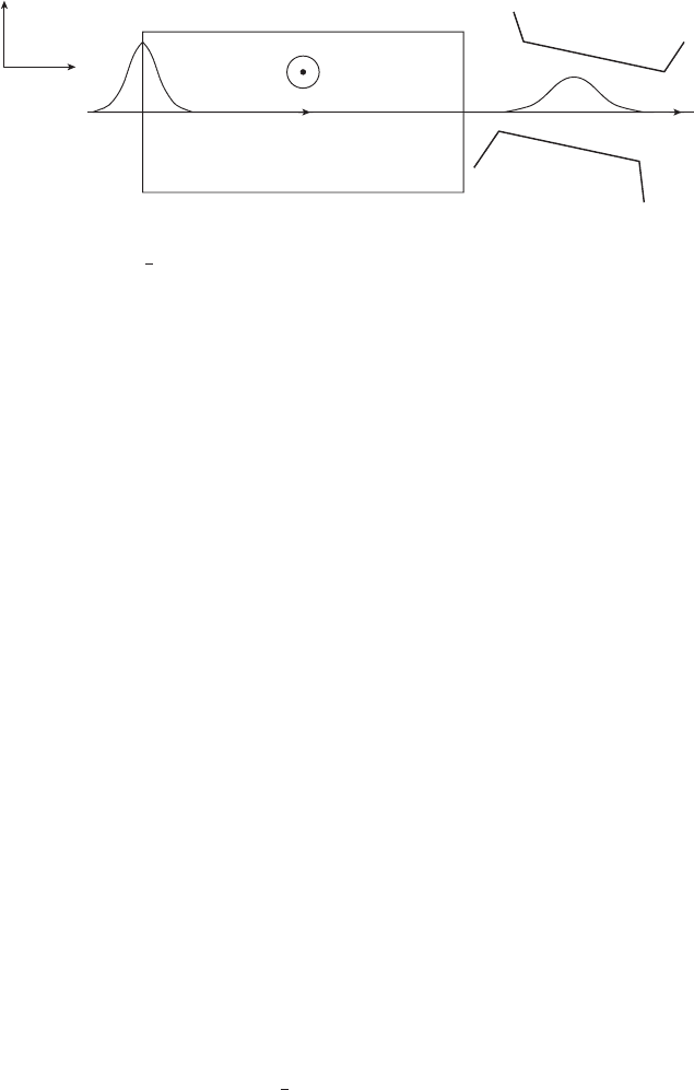
FIGURE 8.1 Spin-

particles, say, neutrons with initial spin orientations polarized along the

x-axis and associated with a localized Gaussian wave-packet (peaked at x = 0, t = 0) pass

through a spin-rotator (SR) containing a constant magnetic ﬁeld B directed along the +

z-axis.

The particles emerging from the SR have a distribution of their spins oriented along different

directions. Calculation of this distribution function is experimentally tested by measuring the

spin observable along a direction

(

)

in the xy-plane making an angle θ with the initial

spin polarized along the +

x-axis. This is done by suitably orienting the direction

(

)

of the

inhomogeneous magnetic ﬁeld in the Stern–Gerlach

(

SG −

)

device.

mediated by the neutron’s magnetic moment µ as the coupling constant. The angle φ

by which the direction of the initial spin-polarization is rotated is determined by the

time (τ) over which this interaction takes place. Now, if the spatial wave-packet is a

superposition of energy eigenstates (plane waves), there will be a distribution (Π(τ))

of times τ over which the interaction between neutron spins and the enclosed mag-

netic ﬁeld takes place, corresponding to the relevant arrival/transit time distribution.

Consequently, using the probability distribution function Π(τ), and an appropriate

relation connecting the quantities φ and τ, one can calculate a distribution of spin

orientations (Π(φ)) for the neutrons emerging from the SR. It is, therefore, evident

that for calculating Π(φ), the quantum mechanical evaluation of Π(τ) for the neutrons

passing through the SR is a key issue.

We will ﬁrst elaborate on the relevant setup by discussing how the determination

of the quantity Π(φ) can actually be tested by using a SG device. Subsequently, we

will discuss the key ingredients of the Bohmian procedure that can be adopted in the

context of this setup for calculating Π(φ) in terms of Π(t). The subtleties involved

in such a procedure will be critically analyzed and directions for further studies will

be indicated that are required to explore fully the potentiality of this example for

subjecting the Bohmian model to empirical scrutiny.

8.2 THE SETUP

We consider an ensemble of spin-

neutral particles, say, neutrons having magnetic

moment µ. The spatial part of the total wave function is represented by a localized

narrow Gaussian wave-packet ψ

(

x, t = 0

)

(for simplicity, it is considered to be one

118 Quantum Trajectories

dimensional) which is taken to be peaked at x = 0 at the initial instant t = 0 and

moves with the group velocity u. Thus the initial total wave function is given by

Ψ = ψ

(

x, t = 0

)

⊗χ

(

t = 0

)

where χ

(

t = 0

)

is the initial spin state which is taken

to be the same for all members of the ensemble oriented along the

x-axis.

The SR used in our setup (Figure 8.1) has within it a constant magnetic ﬁeld

B = B

z directed along the +

z-axis, conﬁned between x = 0 and x = d. We consider

a speciﬁc situation where the magnetic ﬁeld is turned on while the peak of the initial

wave-packet reaches the position x = 0att = 0.

Application of the Larmor precession of spin in a magnetic ﬁeld has earlier been

discussed, for example, in the context of the scattering of a plane wave from a potential

barrier [66,67]. On the other hand, the scheme proposed here explores an application

of Larmor precession such that one can empirically test any given quantum mechan-

ical formulation for calculating the arrival/transit time distribution using a Gaussian

wave-packet.

Now, for testing the scheme for calculating the probability density function Π(φ)

of spin orientations of particles emerging from the SR, we consider the measurement

of a spin variable, say

, by a SG device (Figure 8.1) in which the inhomoge-

neous magnetic ﬁeld is oriented along a direction

(

)

in the xy-plane making an

angle θ with the initial spin-polarized direction (+

x-axis) of the particles. The initial

x-polarized spin state can be written in terms of the z-bases |↑

and |↓

χ(0) = 1/

√



|↑

+|↓



. While passing through the SR, the spin-polarized

state rotates only in the xy-plane by an angle φ with respect to the initial spin orienta-

tion along the

x-axis. Such a rotated spin state in the xy-plane can be typically written

as χ(φ) = 1/

√



|↑

+ e

iφ

|↓



. If one applies the SG-magnetic ﬁeld along

the direction

(

)

, the relevant basis states corresponding to the spin operator ˆσ

are

respectively |↑

= 1/

√



|↑

+ e

iθ

|↓



and |↓

= 1/

√



|↑

− e

iθ

|↓



Then for such spin measurements, the probabilities of getting |↑

and |↓

are

(θ) =|

↑| χ(φ)|

= cos

(θ −φ)/2 and p

−

(θ) =|

↓| χ(φ)|

= sin

(θ −φ)/2

respectively.

8.3 THE TESTABLE PROBABILITIES

Since we are considering an ensemble of spin-

neutrons passing through the SR

where initially all members of this ensemble have their spins polarized along, say, the

x-axis, the spins of individual members of the ensemble evolve over different times

(characterized by Π(t), the distribution of transit times within the SR) of duration of

the interaction with the constant magnetic ﬁeld within the SR.

Thus, for the spins of the particles emerging from the SR polarized along differ-

ent directions (with the respective probabilities Π(φ) of making angles φ with the

x-axis), the probabilities of ﬁnding the spin component along +θ direction and that

along its opposite direction are respectively given by

(

)





Π(φ) cos

(

θ − φ

)

dφ (8.1)

Empirically Probing the Bohmian Model 119

−

(

)





Π(φ) sin

(

θ − φ

)

dφ (8.2)

where P

(

)

+ P

−

(

)

= 1, and n



is any positive number.

It is these probabilities P

(

)

and P

−

(

)

which constitute the actual observable

quantities in our scheme which are determined by the distribution of spins Π(φ)of

the particles emerging from the SR. The theoretical estimations of these probabilities

crucially depend on how one calculates the quantity Π(φ) whose evaluation, in turn, is

contingent on the approach adopted for calculating the relevant time distribution Π(t)

mentioned earlier. Now, the important point to stress here is that the speciﬁcation of

such a time distribution is not unique in quantum mechanics. For the setup indicated

in Figure 8.1, Π(t) represents the arrival time distribution at the exit point

(

x = d

)

of the SR, which is also the distribution of transit times(t) as well as the distribution

of times of interaction with the magnetic ﬁeld within the SR. Thus, Π(t) determin-

ing Π(φ) is the key quantity which needs to be evaluated ﬁrst. In the following

section we focus on discussing the Bohmian procedure for calculating Π(t) leading

to Π(φ).

8.4 THE EVALUATION OF Π(t ) AND Π(φ) USING

THE BOHMIAN MODEL

In the Bohmian model [2–4, 7–10], each individual particle is assumed to have a

deﬁnite position, irrespective of any measurement.The pre-measured value of position

is revealed when an actual measurement is done. Over an ensemble of particles having

the same wave function ψ, these ontological positions are distributed according to the

probability density ρ =|ψ|

where the wave function ψ evolves with time according

to the Schrödinger equation. For the purpose of the present chapter, the relevant key

postulates of the Bohmian model can be expressed as follows:

(i) An individual “particle” embodying the innate attributes like mass, charge, and

the magnetic moment has a deﬁnite location in space at any instant, irrespective of

whether its position is measured or not. In particular, the pre-measurement value of

position is taken to be the same as the value revealed by a measurement of position,

whatever the measurement procedure may be. However, this feature does not hold

for any other dynamical variable, such as the momentum or spin.

(ii) |ψ|

dx is interpreted as the probability of a particle to be actually present

within a region of space between x and x + dx, instead of Born’s interpretation as

the probability of ﬁnding the particle within the speciﬁed region.

(iii) Consistent with the Schrödinger equation and the equation of continuity being

interpreted as corresponding to actual ﬂow of particles with velocity v(x, t), the

equation of motion of any individual particle is determined by the following equation

v(x, t ) =

J (x, t )

ρ(x, t )

∂S(x, t)

∂t

. (8.3)

120 Quantum Trajectories

Here J (x, t) = ρ(x, t )v(x, t ) is interpreted as the probability current density of actual

particle ﬂow and the wave function is considered in the polar form ψ = Re

iS/

with

ρ = R

where R and S are real functions of position and time. In the context of our

SR example, coming to the question of whether there can be predictions obtained

from the Bohmian model which may allow us to empirically discriminate it from the

standard scheme, we analyze this issue as follows.

Here it should be noted that the Schrödinger expression for the probability current

density is inherently nonunique. This is seen from the feature that if one adds any

divergence-free or constant term to the expression for J (x, t), the new expression

also satisﬁes the same equation of continuity derived from the Schrödinger equation.

However, it has been discussed by Holland [11, 12], followed by others [47–49],

that the probability current density derived from the Dirac equation for any spin-

particle is unique, and that this uniqueness is preserved in the nonrelativistic limit

while containing a spin-dependent term in addition to the Schrödinger expression for

J (x, t ). Accordingly, a modiﬁed Bohmian equation of motion for the spin-

particle

has been proposed [11, 12] which is of the form given by

v(x, t) =

(

∇S(x, t) +∇log ρ(x, t) ×s(t)

)

(8.4)

where s(t) =



χ(t)

σχ

†

(t), χ(t) is the time evolving spin state and the components

σ are the Pauli matrices. The modiﬁed Bohmian equation of motion given by

Equation 8.4 reduces to the original Bohmian form given by Equation 8.3 if

∇S





∇ log ρ

, i.e., when the modulus of the spin-dependent term is negligibly small

compared to the spin-independent term. In our setup, the pertinent parameters (viz.

the magnitude of the magnetic ﬁeld, the initial width and the peak velocity of the

wave-packet) are taken to be such that this condition is satisﬁed. Hence, throughout

this chapter, we will neglect any effect of the spin-dependent term in the modiﬁed

Bohmian equation of motion.

Next, we recall the general question of equivalence between the standard ver-

sion and the Bohmian model of quantum mechanics in predicting the observable

results pertaining to any Hermitian operator which has been much discussed [2–4],

along with some controversy [68–71]. Nonetheless, the central point we may stress

is that, given any example, if and only if the procedure for calculating an observable

quantity is unambiguously deﬁned in both the standard and the Bohmian versions

of quantum mechanics, the very formulation of the Bohmian model guarantees the

equivalence (at least, in the non-relativistic domain) when the (common) formalism

is applied.

Now, coming to our example, for the initial state given by Ψ

(

x, t = 0

)

(

x, t = 0

)

⊗ χ

(

t = 0

)

, the time evolution within SR is subject to the interac-

tion Hamiltonian !µσ.B. Note that as the spins of neutrons interact with the time-

independent constant magnetic ﬁeld, in order to conserve the energy, there will

be changes in the momenta of the spatial parts associated with both the up and

down spin components—these changes occur according to the potential energy of the

Empirically Probing the Bohmian Model 121

spin–magnetic ﬁeld interaction that develops corresponding to the up and down spin

components respectively.

In the setup considered here, the relevant parameters (viz. the initial momentum,

mass, magnetic moment, and the magnitude of the applied constant magnetic ﬁeld)

are chosen to be such that the magnitude of the potential energy ( !µσ.B) that arises

because of the spin–magnetic ﬁeld interaction is exceedingly small (≈10

−9

times)

compared to the initial kinetic energy of the neutrons. This amounts to ensuring the

magnitude of the momenta changes within the SR to be negligibly small compared to

the initial momentum. Consequently, the time evolutions of the spatial and spin parts

can be treated independent of each other, with the spatial wave function evolving

freely within the SR (for the relevant justiﬁcation based on a rigorous treatment, see

Appendix A).

With respect to the setup shown in Figure 8.1, the initial wave function is given by

ψ(x, t = 0) =



2πσ



1/4

exp



−

4σ

+ ikx



(8.5)

where the wave number k = mu/, u being the group velocity and σ

is the initial

width of the wave-packet. Now, since the spatial wave function is considered to evolve

freely within the SR, the freely propagating wave function at any instant t is given by

ψ(x, t ) =

(2πA

)

1/4

exp



−

(x −ut)

4σ

+ ik

(

x − ut/2

)



(8.6)

where

= σ



1 +

it

2mσ



Writing Equation 8.6 in the polar form ψ(x, t ) = R(x, t)e

iS(x,t)/

, and using Equa-

tion 8.3, the Bohmian trajectory equation in this setup for the i-th individual particle

having an initial position x

(0) is given by

(t) = ut + x

(0)



1 + βt

(8.7)

with

β =



and the subscript “i” is used as the particle label.

The Bohmian velocity of the i-th individual particle can then be written as a

function of the initial position by using Equation 8.7. The resulting expression is

given by

, t) =

(t)

= u +

βt



1 + βt

. (8.8)

122 Quantum Trajectories

From the above equation it follows that only those particles initially located around

the peak position of the Gaussian wave-packet at x

= 0 follow the Newtonian

equation of motion. On the other hand, the particles initially located within the front

half (x

=+ve) are all accelerated, while the particles initially lying within the

rear half (x

=−ve) are all decelerated [72]. It can then be seen that there will be

turning points of the Bohmian trajectories provided the following relation is satisﬁed

between the instant t



of the turning point and the Bohmian initial velocity u, given by

u =

βt





1 + β(t



)

(8.9)

where x

is essentially −ve. For the purpose of discussion in this chapter, we consider

the relevant parameters (u and σ

) to be such that the above condition is not satisﬁed,

thereby ensuring that, in our example, the particles do not have any turning point

[73, 74]. Next, in order to proceed with the Bohmian calculation of Π(φ), we focus

on the following two quantities pertaining to neutrons which are initially localized,

say, within an arbitrarily chosen region between x

(0) and x

(0) + dx

(0).

First, we note that the probability of neutrons to be actually localized between x

(0)

and x

(0) + dx

(0) is given by |ψ(x

(0), t = 0)|

(0). Secondly, we consider the

probability of these neutrons to cross the region of the magnetic ﬁeld enclosed in the

SR within the time-interval, say, T and T +dT ; this is denoted by Π

(T )dT where

(T )isthearrival time distribution at the exit point (x = d) of the SR, T being

the time required by the i-th neutron to reach the exit point (x = d) of the SR.

Given the notion of trajectories in the Bohmian model, and taking that all the

neutrons initially localized within x

(0) and x

(0) + dx

(0) ultimately pass through

the entire region of the SR (i.e., all of them cross the exit point (x = d) of the SR,

and none of them re-enters), the above two quantities can be equated so that

(T )dT =|ψ(x

(0), t = 0)|

(0) (8.10)

whence

(T ) =|ψ(x

(0), t = 0)|

(0)

. (8.11)

Note that Equation 8.11 is a very general relation that determines the arrival time

distribution in any causal trajectory model, valid for any form of the initial wave-

packet. In the particular case of a freely evolving Gaussian wave-packet we are

considering here in the context of the Bohmian model, we proceed as follows:

By using Equation 8.7, and replacing t by T , the quantity dx

(0)/dT on the right

hand side of Equation 8.11 is calculated by writing x

(0) in terms of x

(T ). Further,

by invoking the earlier outlined interpretive ingredients (ii) and (iii) of the Bohmian

model, we write the quantity |ψ(x

(0), t = 0)|

in terms of x

(T ). This is done by

using Equation 8.3 for ψ(x, t = 0), replacing the argument “x” of this function by

“x

(0)” for varying “i” corresponding to different initial positions of the neutrons.

Then, putting x

(T ) = d, using both Equation 8.7 and the Schrödinger expression

Empirically Probing the Bohmian Model 123

for the probability current density J (x, t), it can be veriﬁed that Equation 8.11

reduces to

(T ) = J (d, T ) (8.12)

where

J (d, T ) =



2πσ



1/2

exp

−

(

d − uT

)

2σ

u +

(

d − uT

)



+ 

(8.13)

is the current density of neutrons at the exit point(x = d) of the SR. Here σ

is the

width of the wave-packet at the instant T . Note that J (d, t) given by Equation 8.13

is essentially a +ve quantity. Thus, Equation 8.12 shows that the Bohmian arrival

time distribution at x = d is the same as that given by the probability current density

(henceforth designated as PCD) approach [36]; i.e.,

(T ) = Π

PCD

(T ) = J (d, T ). (8.14)

Then comes an important element in our example, viz. the consideration of the

time evolution of the spin state according to an equation that is obtained by decoupling

the position and the spin parts of the Pauli equation (adopting the “approximation”

stated earlier whose justiﬁcation is indicated in Appendix A), given by

!µσ.B χ = i

∂χ

∂t

. (8.15)

Now, we recall that in this particular example, the initial spin of any neutron is

taken to be polarized along the +

x-axis; i.e.,

(

)

→



√



↑



↓





. (8.16)

Then, since the constant magnetic ﬁeld B = B

z within the SR, conﬁned between

x = 0 and x = d, is switched on at the instant (t = 0) the peak of the wave-packet

reaches the entry point (x = 0) of the SR, the time evolved neutron spin state χ

(

)

under the interaction Hamiltonian H =!µσ.B is given by

(

)

= exp



−iHτ





(

)

√

−iωτ



↑



+ e

i2ωτ

↓





(8.17)

where ω = µB/ and τ is the spin–magnetic ﬁeld interaction time; i.e., the time during

which the neutron spin state evolves according to the spin–magnetic ﬁeld interaction

term. Equation 8.17 implies that after a time interval τ, the spin orientation of a

neutron is rotated by an angle φ with respect to its initial spin-polarized direction,

where

φ = 2ωτ. (8.18)