Chattaraj P.K. (Ed.) Quantum Trajectories

Подождите немного. Документ загружается.

Semiclassical

Implementation

of Bohmian Dynamics

Vitaly Rassolov and Sophya Garashchuk

CONTENTS

9.1 Introduction...................................................................................................135

9.2 Globally Deﬁned Approximate Quantum

Potential (AQP) ............................................................................................138

9.3 AQP Dynamics with Balanced Approximation Errors..................................141

9.4 Conclusions...................................................................................................146

Acknowledgments..................................................................................................148

Bibliography ..........................................................................................................148

9.1 INTRODUCTION

In this chapter we justify and explain the use of a semiclassical approach in quan-

tum trajectory dynamics, then show how approximations can be balanced to make

the dynamics stable in time. For simplicity, derivations of Sections 9.1 and 9.2 are

given for one-spatial dimension x for a particle of mass m. Arguments of functions

are omitted where unambiguous. Differentiation with respect to x is denoted as ∇.

Differentiation with respect to a variable other than x is indicated with a subscript.

The multidimensional generalization to an arbitrary coordinate system is given in

Ref. [1].

In the Bohmian formulation [2] the usual time-dependent Schrödinger equation

(TDSE),



−



∇

+ V



ψ(x, t ) = ı

∂ψ(x, t)

∂t

, (9.1)

is transformed by representing the complex time-dependent wavefunction in polar

form,

ψ(x, t ) = A(x, t ) exp





S(x, t)



, (9.2)

where A(x, t) and S(x, t ) are real functions. Identifying the gradient of the phase with

the trajectory momentum,

p(x, t) =∇S(x, t), (9.3)

135

136 Quantum Trajectories

and switching to the Lagrangian frame of reference,

∂

∂t

∇, (9.4)

the TDSE (Equation 9.1) leads to the classical-like equations for a trajectory described

by position x

, momentum p

and action function S

(9.5)

=−∇(V + Q)

x=x

(9.6)

− (V +Q)

x=x

. (9.7)

The term Q denotes the quantum potential,

Q =−



∇

A(x, t )

, (9.8)

entering Equations 9.6 and 9.7 on a par with the external “classical” potential V .

Quantum effects are incorporated into the trajectory dynamics through the nonlocal

quantum force, which depends on the wavefunction amplitude and its derivatives up to

third order. With the exception of eigenstates, Q is singular at the wavefunction nodes,

A(x, t ) = 0, resulting in instability of the quantum trajectories describing quantum-

mechanical (QM) interference. Thus, we pursue the idea of using the Approximate

Quantum Potential (AQP), which captures the leading QM effects yet is cheap to

compute. Calculation of the exact Q for general systems is expensive and inaccurate

due to the inherent instability of exact quantum trajectories.

Evolution of the wavefunction density, A

(x, t ), is deﬁned by the continuity equa-

tion, a counterpart of Equation 9.7, and conserves the probability to ﬁnd a particle in

the volume element dx

associated with each quantum trajectory. In other words, the

trajectory “weight” w(x

) is constant in time [3],

w(x

) = A

)dx

dw(x

)

= 0. (9.9)

In the AQP approach we use Equation 9.9 and do not explicitly compute A(x, t).

Once a wavefunction is represented in terms of trajectories, the expectation values of

x-dependent operators can be readily computed,

ˆo(x)



o(x)A

(x, t )dx =



o(x

(i)

, (9.10)

where the index i enumerates the trajectories. The wavefunction normalization is

explicitly conserved. For time-independent V the total wavefunction energy is con-

stant, but the energy of individual quantum trajectories changes in time due to the

inﬂuence of Q.

Semiclassical Implementation of Bohmian Dynamics 137

In addition to x

and p

fully deﬁning the quantum trajectory, we will also consider

the nonclassical momentum r(x, t),

r(x, t) =

∇A(x, t )

A(x, t )

. (9.11)

Formally, it is complementary to the classical momentum p(x, t), since both arise

from the action of the QM momentum operator on the wavefunction in the polar form

(Equation 9.2)

ˆpψ =



−ı

∇A(x, t )

A(x, t )

+∇S(x, t)



ψ =

(

−ır(x, t) + p(x, t)

)

ψ. (9.12)

Q expressed in terms of r becomes

Q =−





(x, t ) +∇r(x, t)



. (9.13)

The equations of motion of the classical and nonclassical momenta computed along

a trajectory have the same structure of the differential operator on the right-hand side

m∇V (x

) + m

= 



∇



∇r

−m



∇



∇p

. (9.14)

In order to solve TDSE using trajectories, or to visualize the wavefunction dynamics,

an ensemble of trajectories is initialized at t = 0. For each initial position x = x

, the

trajectory weight, w = A

(x,0)dx

, and the classical momentum, p

=∇S(x, 0),

are deﬁned. The trajectories evolve according to Newton’s Equations 9.5 and 9.6.

Computation of the exact Q and its gradient requires derivatives of A(x, t) through

third order. This step is approximated in our semiclassical implementation.

In order to examine the semiclassical regime of the Bohmian trajectory method we

have to deﬁne a classical limit of the quantum equations of motion. This is, in general,

a complicated question [4]. In this chapter we take a practical approach and deﬁne

the classical limit in terms of observables. For a particle of mass m, we deﬁne the

classical limit of a quantum state ψ(x)asm →∞provided the energy, ψ|

H |ψ,is

constant. The averaging ... can be performed over any subset of coordinates (such

as only for translational motion). This requires that the wavefunction density, ψ

∗

ψ,

and the kinetic energy density, −

∇

ψ(2mψ)

−1

, remain unchanged as m →∞.

The reactivity of chemical systems is typically governed by the distribution of energy

in various degrees of freedom. It is natural to deﬁne the classical limit preserving this

distribution.

The term “semiclassical” is widespread in chemistry and physics and generally

means “quantum that is close to classical.” The precise deﬁnition depends on the

context. For a numerical procedure not based on the series expansion of the TDSE,

it is natural to deﬁne the semiclassical method as an approximate method describing

138 Quantum Trajectories

some quantum features, which becomes exact in the classical limit [5]. This is a

stringent requirement, which in practice means that approximations must only be

made for the quantities that are negligible in the m →∞or  → 0 limits, and

that the errors of the method can be controlled, at least in principle. In particular,

removing singularities in the quantum potential by constraining the density, phase,

or momentum would generally violate the semiclassical condition. In contrast, the

AQP method constrains the functional form of the nonclassical momentum r(x, t)

appearing in Equation 9.12 with the  prefactor, while the wavefunction density itself

is unconstrained. Thus, the AQP approach can be systematically improved if the

linearization of the nonclassical momentum is accomplished over subspaces [6] or if

r(x, t) is represented in terms of a complete basis.

9.2 GLOBALLY DEFINED APPROXIMATE QUANTUM

POTENTIAL (AQP)

The point of developing the AQP method is to have an inexpensive, robust semiclas-

sical approach that can be applied to high-dimensional systems. “Inexpensive” means

that the scaling with the system size is polynomial, ideally linear, such that the compu-

tation of the quantum force is a small addition to the classical trajectory propagation.

The polynomial scaling allows the method to be applied to hundreds of degrees of

freedom. “Robust” implies numerical stability. In particular, the numerical propaga-

tion should be insensitive to trajectory crossings—exact quantum trajectories do not

cross (!)—and should switch to classical propagation if the quantum force becomes

inaccurate. “Semiclassical” means that the method should describe the leading QM

effects. However, it should not aim for exact QM dynamics—a necessary trade-off

for a better than exponential scaling with system dimensionality. In addition, it is

desirable for a method to have an accuracy criterion and a systematic procedure for

achieving the exact QM description.

Analytical representation of the (approximate) quantum potential is essential for

efﬁcient and accurate computation of the quantum force. One physically appealing

way of constructing the AQP is to ﬁt the nonclassical component, r(x, t), given by

Equation 9.11. The representation of this single object within a basis

f (x),

r(x, t) ≈˜r(x, t) =!c(t) ·

f (x), (9.15)

can be used to obtain Q and its gradient by using ˜r instead of r(x, t) in Equation 9.13.

The vector !c contains the time-dependent basis expansion coefﬁcients found from the

minimization of a functional

I =



∞

−∞

(r −˜r)

(x, t )dx (9.16)

with respect to the elements of !c. Integrating by parts and replacing integrals

with sums over the trajectories, the solution to this linear minimization problem,

∇

I = 0, is

!c =−

−1

b. (9.17)

Semiclassical Implementation of Bohmian Dynamics 139

The matrix S contains the time-dependent basis function overlaps,

=f

=



x=x

(i)

(9.18)

and the vector

b consists of averages of ∇f ,

=∇f

=



x=x

(i)

. (9.19)

As shown in Ref. [7], AQP evaluated for expansion coefﬁcients given by Equa-

tion 9.17 conserves the total energy of a system.

The smallest physically meaningful basis

f consists of just two functions

f = (1, x), in which case, the approximation is particularly transparent,

˜r =−

x −x

2(x

−x

)

. (9.20)

For normalized wavefunctions the nonclassical momentum is approximated with

a linear function centered at the average position of the wavepacket with the slope

inversely proportional to the variance, σ =x

−x

.This functional form of ˜r deter-

mines the quadratic AQP and, consequently, the linear quantum force—thus the name

Linearized Quantum Force (LQF). The force is inversely proportional to σ

and, there-

fore, quickly vanishes for spreading wavepackets. From the physical point of view, the

linear nonclassical momentum exactly corresponds to a Gaussian wavepacket evolv-

ing in time in a locally quadratic potential. For general potentials, it can describe

the dominant quantum effects in semiclassical systems, such as wavepacket bifurca-

tion, wavepacket spread in energy, and moderate tunneling. Zero-point energy (ZPE)

effects are reproduced for short times—a few vibrational periods and depending on

the anharmonicity of the system, which is adequate for direct gas phase reactions.

For instance consider photodissociation of ICN described within the two-

dimensional Beswick–Jortner model [8] (see Ref. [9] for details). A wavepacket

representing the ICN molecule is promoted by a laser from the ground to the

excited electronic state, where the molecule dissociates into I and CN. The initial

wavefunction

ψ(x, y,0)=

(α

− α

)

1/4

−α

(y−¯y)

−α

(x−¯x)

+2α

(y−¯y)(x−¯x)

(9.21)

is deﬁned as the lowest eigenstate of the ground electronic surface composed of the

harmonic potentials in CN and CI stretches. Thus, ψ(x, y, 0) is a correlated Gaussian

wavepacket located on the repulsive wall of the excited surface. The photodissociation

spectrum is computed from the Fourier transform of the wavepacket autocorrelation

function C(t),

I (E) =



∞

−∞

C(t)e

ıEt

dt, C(t) =ψ(0)|ψ(t).

140 Quantum Trajectories

For real ψ(x, y, 0), C(t) can be written as

C(t) =ψ(−t/2)|ψ(t/2)=ψ

∗

(t/2)|ψ(t/2)=



exp(2ıS

(i)

t/2

). (9.22)

Note, that in Equation 9.22 we need only half the propagation time, which improves

accuracy.

The physical value of the repulsion parameter of the excited potential surface yields

a rather simple dissociation dynamics; C(t) decays on the time-scale of about one and

a half oscillations of the CN stretch, and the LQF spectrum is in excellent agreement

with the quantum result [10]. The repulsion parameter, three times larger than its

physical value, leads to predissociation processes providing a more challenging test

(system II in Ref. [9]). As detailed in Ref. [7], in two dimensions the nonclassical

momentum is a vector, !r = (r

(x)

, r

(y)

). In the LQF treatment, both components of !r are

approximated in a linear basis

f = (1, x, y) with the component-speciﬁc expansion

coefﬁcient vectors ˜r

(x,y)

f ·!c

(x,y)

. The minimization procedure is analogous to the

one-dimensional case,

∇

I =∇

I = 0, I =(r

(x)

−˜r

(x)

)

+(r

(y)

−˜r

(y)

)

. (9.23)

The solution is Equation 9.17 with the vectors !c and

b replaced with matrices

C = (!c

(x)

, !c

(y)

), and B = (∇

f , ∇

f ), respectively.

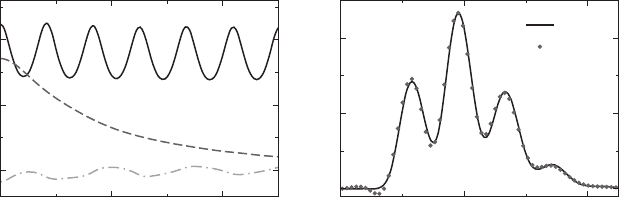
The wavefunction was represented by an ensemble of 167 trajectories propa-

gated for three vibrational periods of the CN stretch. The LQF parameters describing

wavepacket localization are shown in Figure 9.1a: c

(x)

represents the changing width

of the wavepacket in the CN mode; c

(y)

describes the wavepacket spreading in the

dissociation mode; c

(x)

= c

(y)

reﬂects the correlation between the degrees of free-

dom. Figure 9.1b compares the semiclassical spectrum computed using Equation 9.22

with the result of the exact QM wavepacket evolution. The accuracy of the LQF cor-

relation function deteriorates at long times, which is manifested in small errors of its

0 1000 2000

Time

100

LQF parameters

(a) (b)

0 0.02 0.04

Energy

I(E)

LQF

FIGURE 9.1 ICN dissociation. (a) The LQF wavepacket width parameters: c

(x)

(solid line),

(y)

(dash), and c

(x)

= c

(y)

(dot-dash). (b) The Fourier transform of the correlation function.

The LQF result is computed using Equation 9.22.

Semiclassical Implementation of Bohmian Dynamics 141

Fourier transform for low energies. Nevertheless, the overall agreement of the spectra

is quite good, demonstrating that LQF is sufﬁciently accurate for systems with fast

dynamics.

There are several ways to improve the description of non-Gaussian wavefunctions

evolving in general potentials. The LQF parameters can be optimized on subspaces

representing, for example, the reaction channels [6]. More functions can be added to

the basis

f . For example, the Chebyshev basis of up to six polynomials has been used

in Ref. [11]. Small bases can be tailored to the system. For example, a two-function

basis consisting of a constant and an exponent gives an exact description of r for the

eigenstate of the Morse oscillator as used in Ref. [12] to describe the ZPE of H

in the

reaction channel of the O+H

reaction.Amixed coordinate-space/polar wavefunction

representation can be employed to describe hard QM effects, such as wavefunctions

with nodes and nonadiabatic dynamics [13–15]. For condensed phase dynamics we

developed a stabilized version of the LQF as it is cheap in many dimensions [16].

9.3 AQP DYNAMICS WITH BALANCED APPROXIMATION ERRORS

Most often a reaction occurring in a condensed phase is represented by a reactive

coordinate coupled to a molecular environment or a “bath.” The main QM effects

that can be signiﬁcant in such a system are (i) the motion along the reactive coor-

dinate possibly inﬂuenced by QM tunneling and (ii) the ZPE—or, more generally,

localization energy—in the reactive and bath degrees of freedom and energy ﬂow

among them. The energy changes in the reactive mode will obviously inﬂuence the

probability of the reaction.

Formally, the ZPE is the energy of the lowest eigenstate. It is a sum of the kinetic and

potential energy contributions due to localization, or “ﬁnite size,” of the eigenstate.

In the Bohmian formulation, the kinetic energy contribution to the ZPE is given by

the expectation value of the quantum potential,

Q=−



A|∇

A=



∇A|∇A=



r

. (9.24)

It can be called the “quantum” energy in contrast to the “classical” energy, p

2m +V . The concept of “quantum” energy can be applied to any localized function,

not just to the ground state. An efﬁcient—scalable to high dimensionality—and stable

description of the quantum energy, Q, is the goal of this section.

The LQF approximation gives the exact quantum energy for all eigenstates and

coherent states of the harmonic oscillator. In anharmonic systems, the LQF describes

Q only on a short time-scale (depending on the anharmonicity). For an eigenfunc-

tion in the Bohmian formalism, the quantum force exactly cancels the classical one

resulting in stationary trajectories. In the LQF, exact cancellation generally does not

happen; a net force acting on the trajectories, representing the wavefunction tails,

might be large causing these “fringe” trajectories to start moving. Sooner or later,

the movement will affect the moments of the trajectory distribution resulting in a

decoherence of the LQF trajectories and in a loss of the ZPE (or quantum energy)

142 Quantum Trajectories

description. Since the total energy is conserved, the quantum energy will be trans-

ferred into the classical energy of the trajectory motion. Below, the LQF ideas are

extended to prevent this “loss” of quantum energy for small anharmonicities, or more

precisely for small nonlinearity of the classical and nonclassical momenta. Thus, a

cheap and stable ZPE description over many oscillation periods is provided.

The derivation is given in atomic units ( = 1) for a system described in N

dim

Cartesian coordinates !x = (x, y, ...) in vector notation. The classical and nonclassi-

cal momenta are vectors

!p =∇S, !r = A

−1

∇A. (9.25)

In LQF, a linear approximation to each component of A

−1

∇A is made. The trajectory

momenta are known but never used in the ﬁtting procedure. The nonlinearity of !p,

however, quickly translates into nonlinearity of !r. In this section, !r and !p are treated

on an equal-footing. The deviations of both quantities from linearity are used to limit

the accumulation of propagation errors with time.

In the multidimensional case, the time-evolution of !r and !p along a trajectory,

given by Equation 9.14 in one dimension, is:

m∇V +m

d !p

= (!r ·∇)!r +

(∇·∇)!r

−m

d!r

= (!r ·∇) !p +

(∇·∇) !p

. (9.26)

For practical reasons the spatial derivatives of !r and !p in Equations 9.26 need to be

determined from the global approximations to these quantities. The trajectory-speciﬁc

quantities !r and !p are found by solving Equations 9.26. In general, the relations in

Equation 9.25 are not fulﬁlled once approximations are made to the right-hand sides

of Equations 9.26. As in LQF, !p and !r are expanded in a basis set of functions for the

purpose of derivative evaluations. The expansion coefﬁcients are determined from

the minimization of the error functional using the total energy conservation as a

constraint.

The total energy can be deﬁned without spatial derivatives as

E =

!p ·!p

+V +

!r ·!r

. (9.27)

The energy conservation constraint will couple the ﬁtting procedures of A

−1

∇A

and !p. The linear basis

f =(x, y, ..., 1) is considered here. Formulation for a general

basis is given in Ref. [16]. The functions

{˜r

=!c

f , ˜r

=!c

f , ...} (9.28)

approximate components of the vector A

−1

∇A. The functions

{˜p

=!c

f , ˜p

=!c

f , ...} (9.29)

Semiclassical Implementation of Bohmian Dynamics 143

approximate components of the vector !p. In order to express the energy conservation

condition, dE/dt = 0, the ﬁtting coefﬁcients are arranged into matrices C

and C

=[!c

, !c

, ...], (9.30)

=[!c

, !c

, ...]. (9.31)

Differentiating Equation 9.27 with respect to time and using Equations 9.26 with

the derivatives obtained from Equations 9.28 and 9.29, the energy conservation con-

dition becomes

!r

· (C

!p − C

!r)

= 0. (9.32)

The quantity !r

denotes a vector of nonclassical momentum extended to the size of

the basis N

dim

+ 1

= (r

, r

, ..., 0). (9.33)

The matrices C

and C

are symmetric.

The least squares ﬁt of A

−1

∇A and !p in terms of a linear basis with the constraint

Equation 9.32 is minimization of the functional

I =&A

−1

∇A − C

f &

+&!p − C

f &

+2λ!r

· (C

!p − C

!r) (9.34)

with respect to the ﬁtting coefﬁcients and with respect to the Lagrange multiplier λ.

The optimal coefﬁcients solve a system of linear equations,

























. (9.35)

In Equation 9.35 the following matrices and vectors are introduced: (i) M is the

block-diagonal matrix of the dimensionality N

dim

×N

dim

with the basis function

overlap matrix S =

f ⊗

f  as N

dim

blocks on the diagonal and zeros otherwise;

(ii) O is a zero matrix of the same size as M; and (iii) the elements of the vectors

, and

are the elements of the matrices C

, C

, B

, D

and D

, respectively, listed in column-by-column order. C

and C

are given by

Equations 9.30 and 9.31. The remaining four matrices are deﬁned as

=−

(∇⊗

f )

, B

=

f ⊗!p (9.36)

=−!r

⊗!r, D

=!p

⊗!r, (9.37)

where !p

denotes a vector of classical momentum extended to the size of the basis

=(p

, p

, ..., 0). (9.38)