Cain G., Meyer G.H. Separation of Variables for Partial Differential Equations: An Eigenfunction Approach
Подождите немного. Документ загружается.

page_122
file:///G|/%5EDoc%5E/_new_new/got/020349878X/files/page_122.html[22/02/2009 23:52:36]
< previous page page_122 next page >
Page 122
But these functions are linearly independent. (Their Wronskian at
t=
0 is the nonzero determinant of a
Vandermonde matrix.) Hence there is no interval [0,
T
] for
T>
0 such that
In other words, the thermal signal generated by the boundary condition
u
(
t,
0)=1,
t
>0,
is felt immediately at
L
=1. Thus the thermal signal travels with infinite speed through [0,
L
]. This
phenomenon was already observed in Section 1.4 and is a well-known consequence of Fourier’s law of
heat conduction. It contradicts our experience that it will take time before the heat input at
x=
0 will be
felt at
x=L.
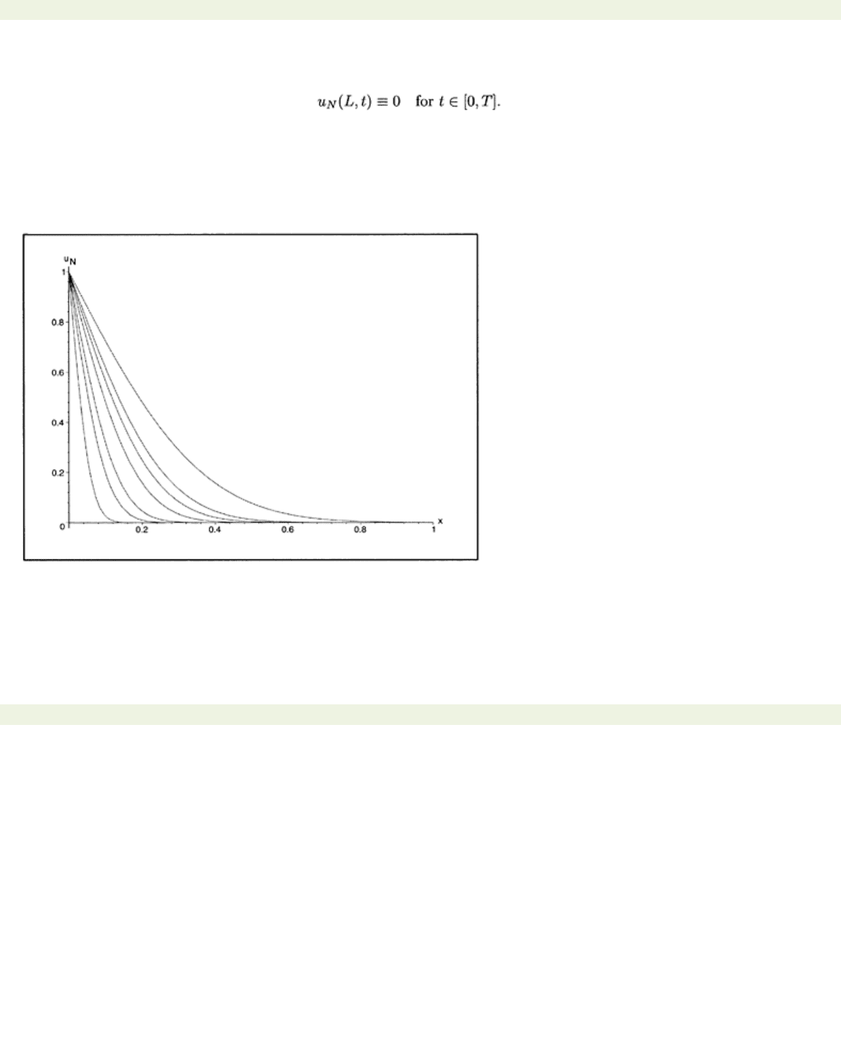
But in fact, for all practical purposes a detectable signal does travel with finite speed. Fig.
6.3a shows a plot of
uN(x, t)
for a few values of
t.
Figure 6.3: (a) Plot of
uN(x, t)
for increasing
t.
We see a distinct thermal wave moving through the interval. We can use (6.2) to compute the speed
with which an isotherm moves through the interval. We shall set
L=
1 and determine the speed
s′(t)
of
the isotherm
uN(s(t), t)=
.001.
Specifically, for given
xi=i
/100,
i
=10,…, 99 we shall compute first the time
t=T(xi)
when the isotherm
reaches
x
i
. T(xi)
is found by applying Newton’s
< previous page page_122 next page >
page_123
file:///G|/%5EDoc%5E/_new_new/got/020349878X/files/page_123.html[22/02/2009 23:52:36]
< previous page page_123 next page >
Page 123
method to the nonlinear equation
F(y)=uN(x
i
, t)−
.001=0
where
y
=
et
and
uN(x, t)
is given by (6.2) so that
Once
T(xi)
is known the speed
s′(T(xi))
of the isotherm at
xi
can be determined from
for
s(t)=xi
and
t
=
T(xi).
The partial derivatives of
uN
are available from (6.2).
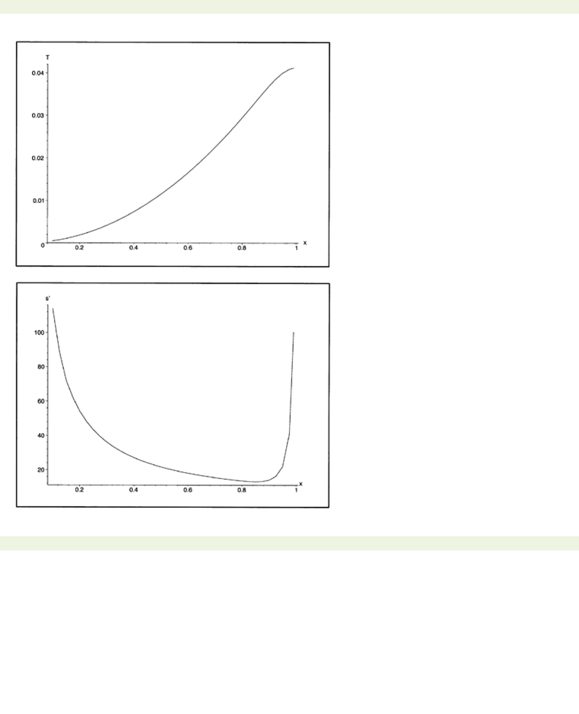
Figs. 6.3b, c show
T(xi)
and
s′(t)
for points in the interval (0, 1).
The answers remain unchanged for
N
>50. However, we need to point out that we begin our calculation
at
x=
.1. For
x<
.1 the initial Gibbs phenomenon causes very slow convergence of the series (6.2)
because
t=T(x)
is small. This makes the calculation of
T(x)
difficult and the answers unreliable.
However, because the answer is analytic, this initial effect does not pollute the answer at later times and
other locations.
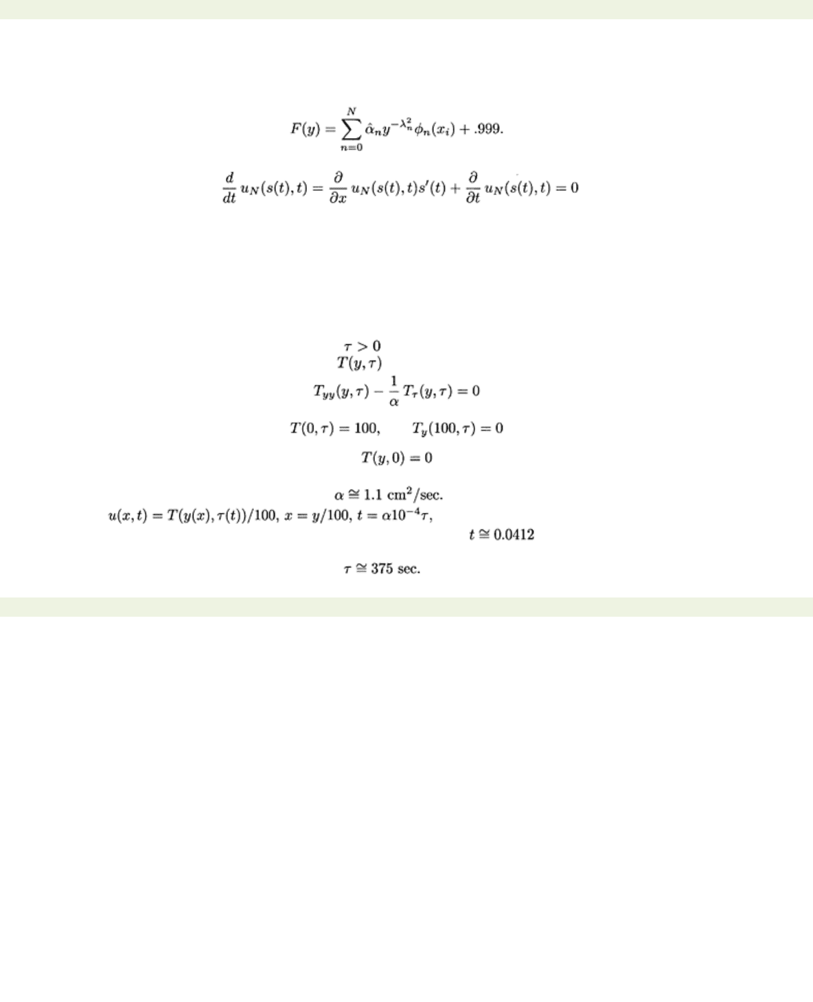
To give meaning to these numbers suppose aim copper rod is insulated along its length and at its right
end. Its initial temperature is 0°C. For time its temperature at the left end is maintained at 100°
C. The thermal model for the temperature
in the rod is
where a is the diffusivity of copper, given in [19] as
If we write then
u
satisfies the equations of this example.
The isotherm
u=
.001 (i.e.,
T=
.1°C) reaches the right end at which corresponds to a real time
of
< previous page page_123 next page >
page_124
file:///G|/%5EDoc%5E/_new_new/got/020349878X/files/page_124.html[22/02/2009 23:52:37]
< previous page page_124 next page >
Page 124
Figure 6.3: (b) Arrival time
T
of the isotherm
u=
.001 at
x.
Figure 6.3: (c) Speed
s′
of the isotherm
u=
.001 at
x.
< previous page page_124 next page >
page_125
file:///G|/%5EDoc%5E/_new_new/got/020349878X/files/page_125.html[22/02/2009 23:52:38]
< previous page page_125 next page >
Page 125
Conversely, the transient part of the solution will have decayed at the end of the rod to −.001 when
which yields
t=
2.89 and a real time of The additional terms of the transient solution are
negligible for such large
t.
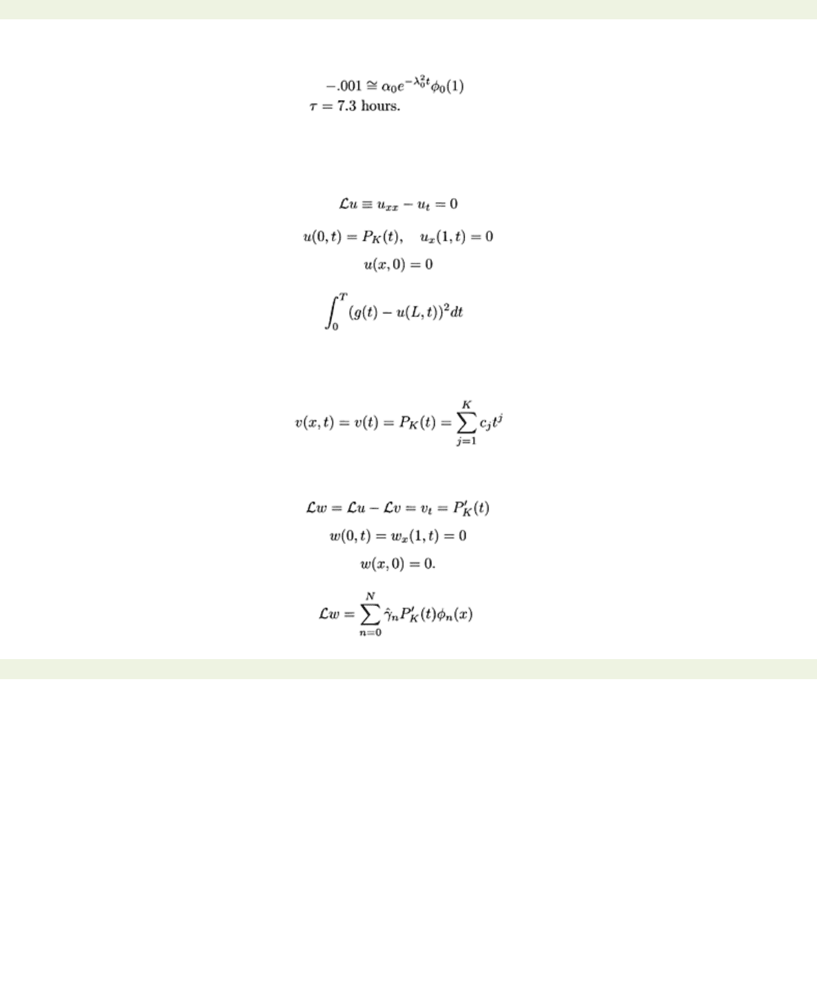
Example 6.4 Matching a temperature history.
We shall determine a heating schedule at
x=
0 to match a desired temperature at the end of a perfectly
insulated slab or bar. Specifically, we shall find a polynomial
PK(t)
with
PK
(0)
=
0 such that the solution
u(x, t)
of
minimizes the integral
where
g
is a given target function and
T
is fixed.
In general, this is a difficult problem and may not have a computable solution. However, the
corresponding approximating problem is straightforward to solve.
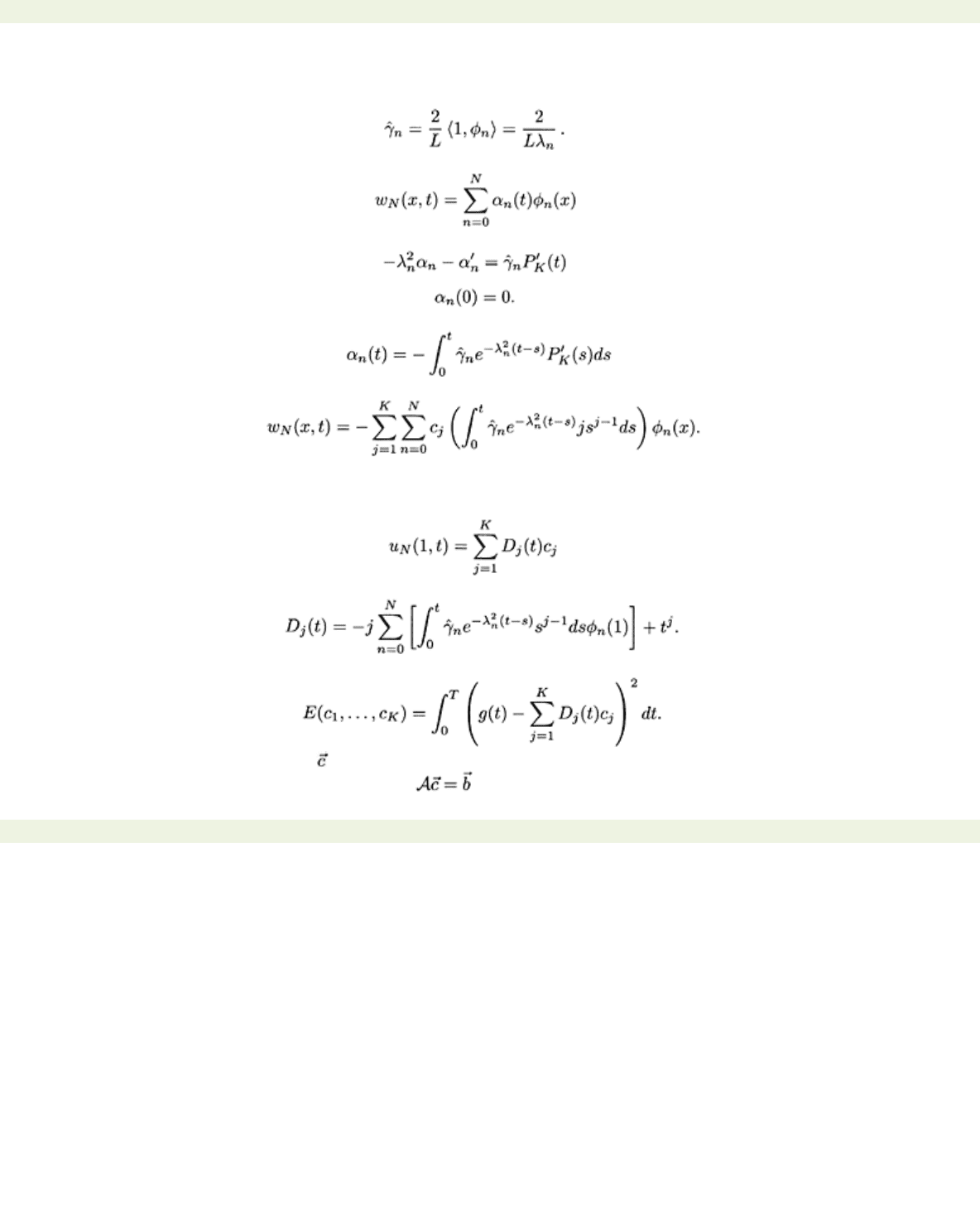
The boundary conditions are zeroed out if we choose
where the
{cj}
are to be determined. Then
w(x, t)=u(x, t)−v(t)
satisfies
The associated eigenvalue problem is the same as in Example 6.2, and the approximating problem is
< previous page page_125 next page >
page_126
file:///G|/%5EDoc%5E/_new_new/got/020349878X/files/page_126.html[22/02/2009 23:52:39]
< previous page page_126 next page >
Page 126
w
(
x,
0)=0
where
The problem is solved by
where
The variation of parameters solution is
so that
Hence the approximate solution
uN(x, t)=wN(x, t)
+
PK(t)
at
x
=1 is
where
It is now straightforward to minimize
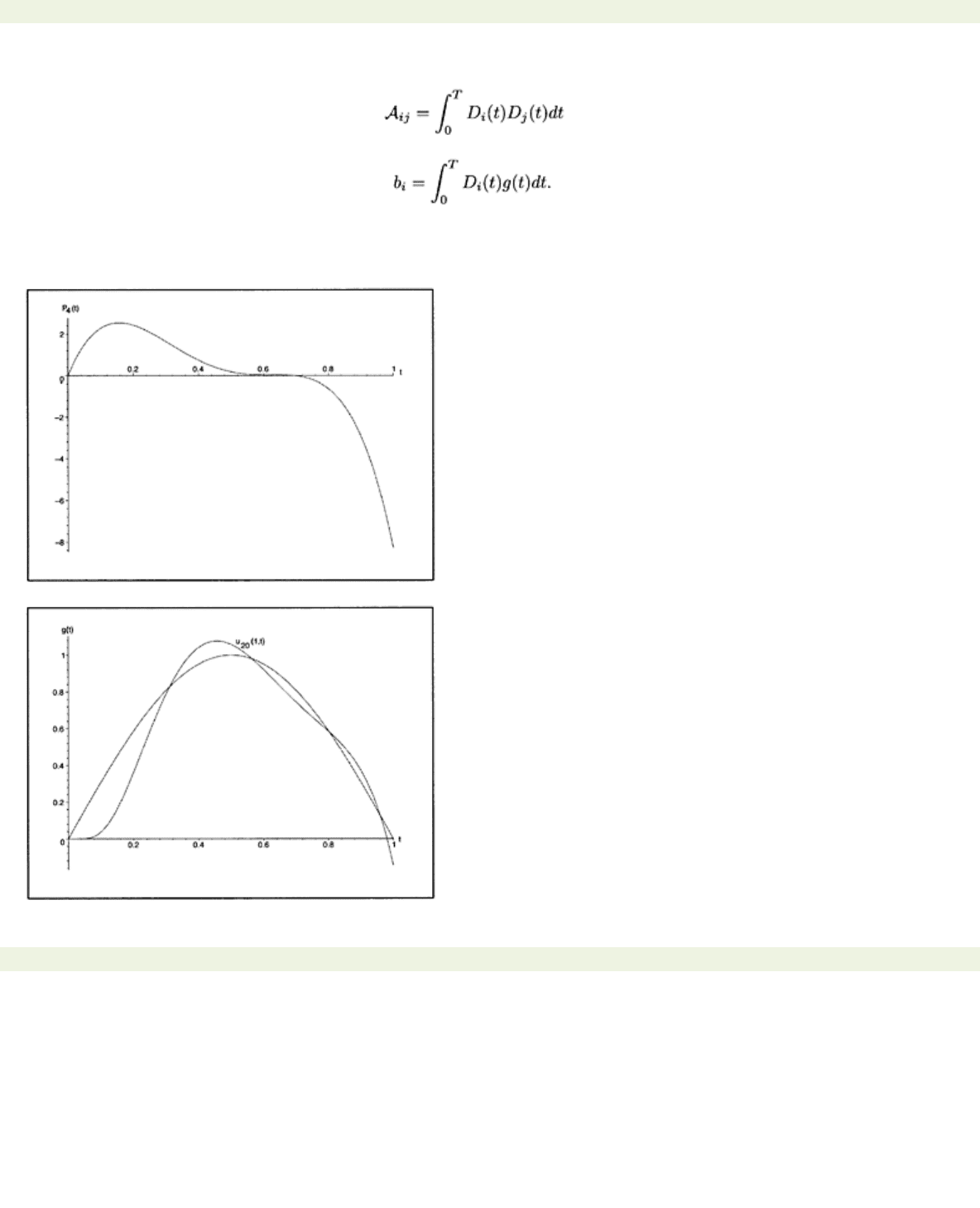
Calculus shows that the solution is found from the matrix system
< previous page page_126 next page >
page_127
file:///G|/%5EDoc%5E/_new_new/got/020349878X/files/page_127.html[22/02/2009 23:52:39]
< previous page page_127 next page >
Page 127
where
and
For a representative calculation we choose
L=T
=1 and try to match
g(t)=
sin
πt
.
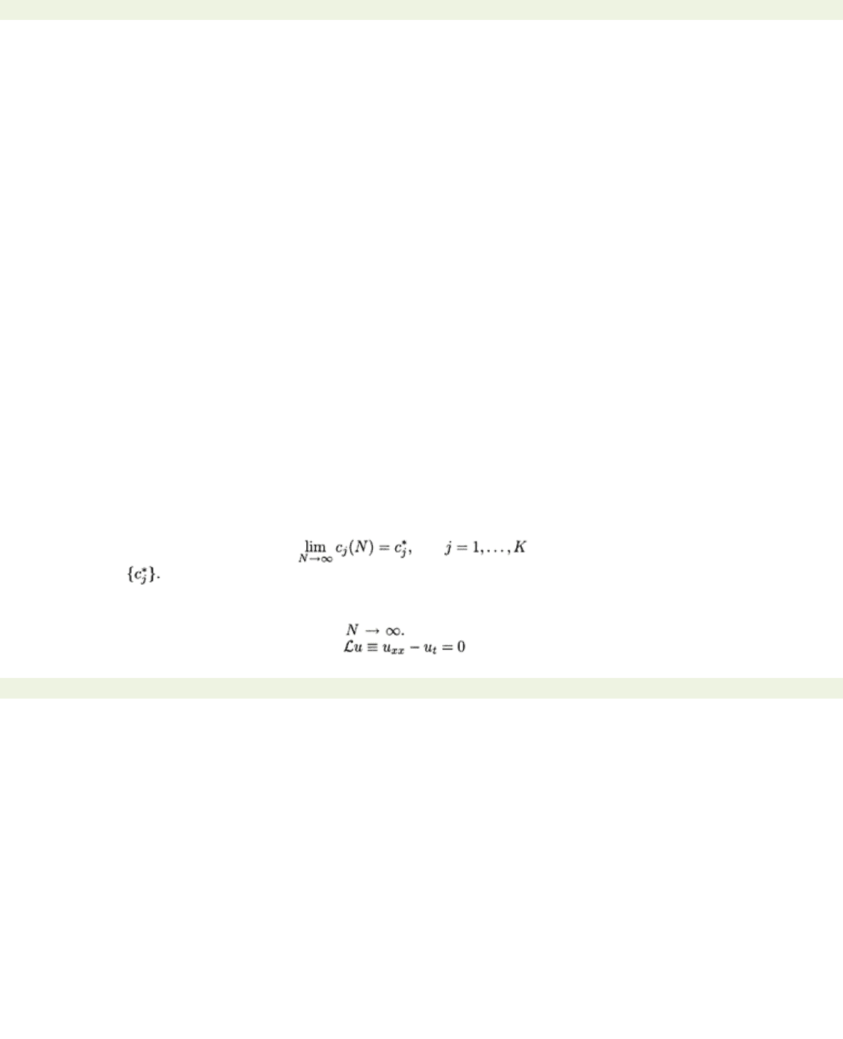
Fig. 6.4a shows the optimal polynomial
P
4
(t)
while Fig. 6.4b shows the target function
g(t)
and the
computed approximation
uN(x, t)
for
N=
20.
Figure 6.4: (a) Computed polynomial
P
4
(t)
for the boundary condition
u
(0,
t
)
P(t).
Figure 6.4: (b) Plot of
u
20(1,
t
) and the target function
g(t)=sm πt.
< previous page page_127 next page >
page_128
file:///G|/%5EDoc%5E/_new_new/got/020349878X/files/page_128.html[22/02/2009 23:52:40]
< previous page page_128 next page >
Page 128
The computation was carried out with Maple which automatically performs all calculations symbolically
where possible and numerically otherwise. In this language the entire problem took no more
programming effort than writing the above mathematical expressions in Maple notation. To illustrate this
point we list below the entire Maple program leading to the graphs in Figure 6.4a, b.
> with (Linear Algebra): with (plots):
> lambda:=n->(2*n+1)*(Pi/2);
> phi:=(x,n)->sin(lambda(n)*x);
> g:=n->integrate(phi(x,n),x=0..1)/integrate(phi(x,n)^2,x=0..1);
> F:=(t,N,k)->k*add(–g(n)*integrate(exp((s–t)*lambda(n)^2)*
(s^(k–1)), s=0..t)* phi(1, n), n=0..N)+t^k;
> a:=(j,k)->integrate(F(t,N,k)*F(t,N,j),t=0..T);
> b:=j->integrate(B(t)*F(t,N,j),t=0..T);
> N:=10;K:=4;T:=1;
> B:=t->sin(Pi*t);
> AA:=evalf(Matrix(K,K,(j,k)->a(j,k)));
> RS:=evalf(Matrix(K,1,(j)->b(j)));
> COE:=LinearSolve(AA,RS);
> P:=t->add(COE[j, 1]*t^j,j=1..K);
> plot(P(t),t=0..1);
> PP:=t→add(j*COE[j,1]*t^(j−1),j=1..K);
> alpha:=(t,n)->−g(n)*integrate(PP(s)*exp(-(t-s)*
lambda(n)^2), s=0..t);
> u:=t->add(alpha(t,n)*phi(1,n),n=0..20)+P(t);
> p1:=plot(u(t),t=0..1):p2:=plot(B(t),t=0..1):
> display(p1, p2);
The above calculation yields a polynomial of degree
K
whose coefficients
cj
clearly depend on the
dimension of the subspace in which the solution
wN(x, t)
is found, i.e.,
cj=cj(N).
In order for the answer
to remain meaningful for the original problem, we would need a proof that
for constants
We do not have such a result but take assurance from numerical experiments that
show that
P
4
(t)
changes little for
N>
10.
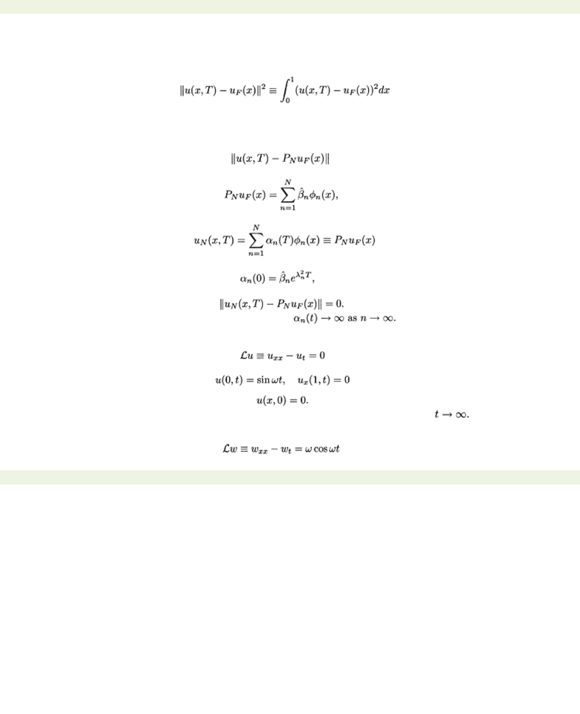
Such a behavior cannot always be expected, and it may well be that a problem is solvable in the
subspace but that the answers diverge as For example, consider the following problem:
< previous page page_128 next page >
page_129
file:///G|/%5EDoc%5E/_new_new/got/020349878X/files/page_129.html[22/02/2009 23:52:41]
< previous page page_129 next page >
Page 129
u
(0
, t
)
=ux
(1
, t
) =0
u
(
x
,0)=
u
0(
x
)
where
u
0 is to be determined such that
is minimized for a given target function
uF.
This formulation is actually a disguised way of writing an
initial value problem for the backward heat equation which, we know from Section 1.4, is a notorious ill-
posed problem. If
uF(x)
is projected into the subspace spanned by the first
N
eigenfunctions of the
associated Sturm-Liouville problem, i.e., if we wish to find
u
0
(x)
such that
is minimized where
then
if
i.e., we have
But
uN
does not converge for
t<T
as
N
→
∞
because
Example 6.5 Phase shift for a thermal wave.
Consider the problem
It is reasonable to expect that
u
(1,
t
) will vary sinusoidally with frequency
ω
as Our aim is to
find the phase shift of
u
(1,
t
) relative to
u
(0,
t
).
To zero out the boundary data we set
w(x, t)
=
u(x, t)−
sin
ωt.
Then
< previous page page_129 next page >
page_130
file:///G|/%5EDoc%5E/_new_new/got/020349878X/files/page_130.html[22/02/2009 23:52:42]
< previous page page_130 next page >
Page 130
w
(0
, t
)
=wx
(1
, t
)=0
w
(
x,
0)
=0.
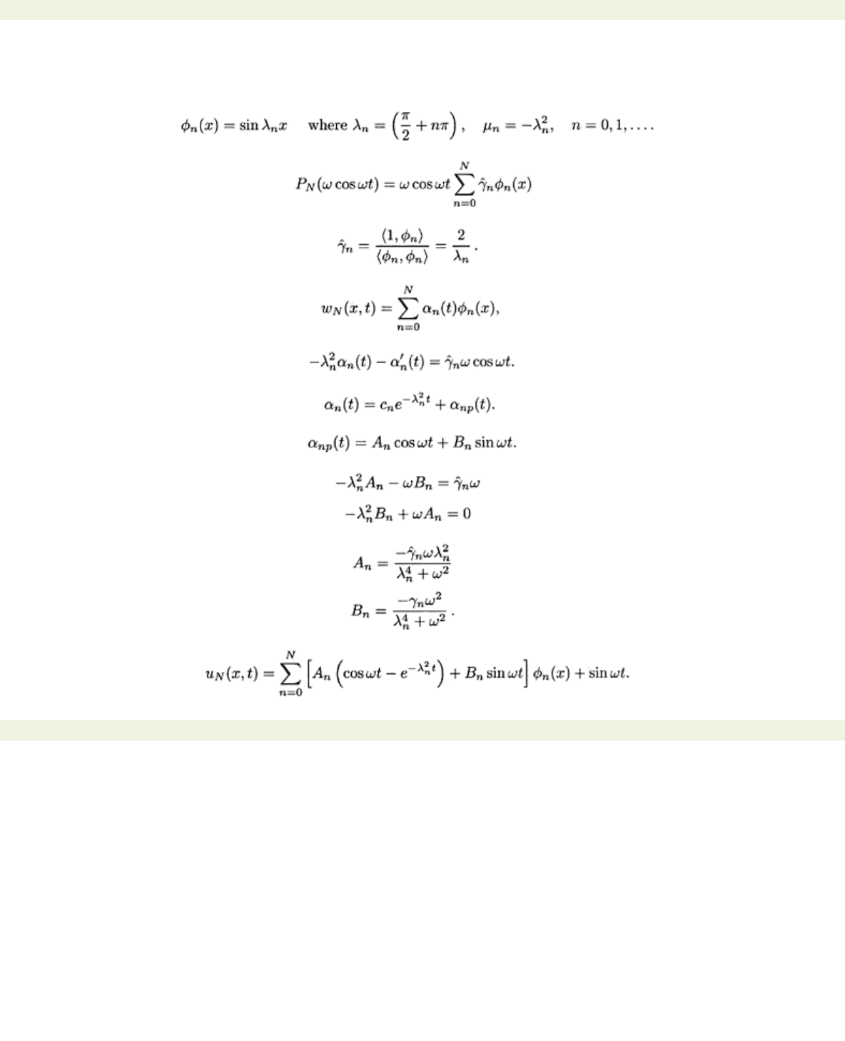
As above the eigenfunctions and eigenvalues are
Then
where
If
then
It follows that
To find a particular integral we use the method of undetermined coefficients and try
Substituting into the differential equation and equating the coefficients of sin
ωt
and cos
ωt
we find
so that
The final approximate answer to our problem is
< previous page page_130 next page >
page_131
file:///G|/%5EDoc%5E/_new_new/got/020349878X/files/page_131.html[22/02/2009 23:52:42]
< previous page page_131 next page >
Page 131
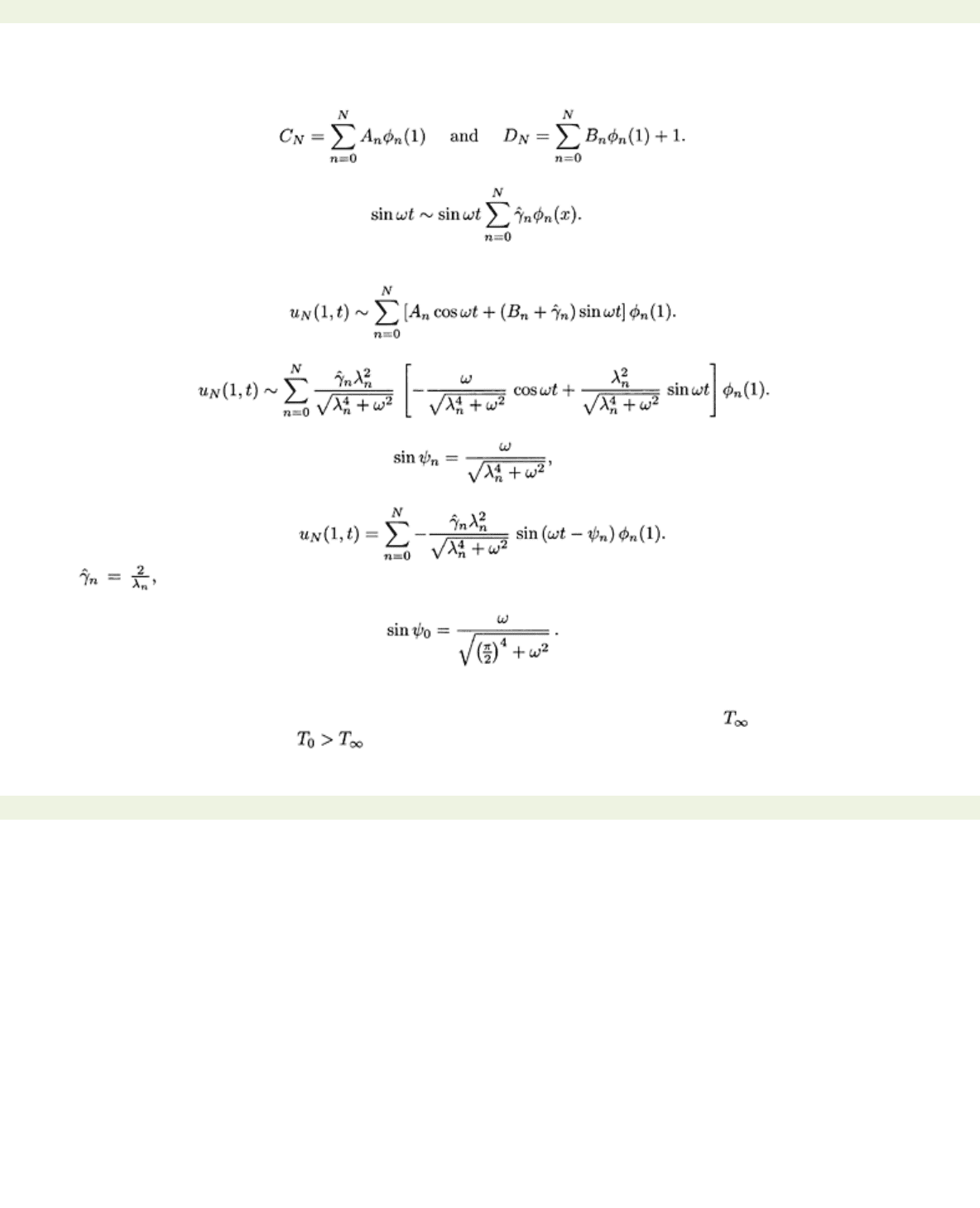
The exponential terms decay rapidly and will be ignored. It is now straightforward to express the phase
shift in terms of
However, perhaps more revealing is the following approach. We write
This is the Fourier series of the four-periodic odd function which coincides with sin
ωt
on (0, 2). This
series converges uniformly near
x=
1. Ignoring again the exponential terms we can write
This expression can be rearranged into
If we set
then
Since we see that the dominant term corresponds to
n
=0 which yields a phase shift
ψ
0 given
by
Example 6.6 Dynamic determination of a convective heat transfer coefficient from
measured data.
A bar insulated along its length is initially at the uniform ambient temperature
and then heated
instantaneously at one end to
while it loses energy at the other end due to convective cooling.
The aim is to find a heat
< previous page page_131 next page >
