Buschow K.H.J. (Ed.) Concise Encyclopedia of Magnetic and Superconducting Materials

Подождите немного. Документ загружается.

pinning sites for domain wall motion and in this way

generate high coercivities. An overlong aging treat-

ment leads to particle growth so that these are

no longer single-domain particles. Consequently, the

coercivity is reduced.

Investigations by Watanabe (1991) have made it

clear that permanent magnets with hard magnetic

properties even superior to those of CoPt alloys can

be obtained for FePt alloys to which a small amount

of niobium is added. The corresponding ingots are

ﬁrst homogenized at 1325 1C and then quenched in

water. The desired high coercivity is obtained after

a subsequent isothermal annealing treatment per-

formed in a temperature range of 600–700 1C. The

iron moments are somewhat higher than the cobalt

moments in the iron alloys. This implies also that the

remanences in the iron alloys are higher than in the

cobalt alloys. This, in turn, leads to larger maximum

energy products with (BH)

max

values higher than

160 kJm

3

The platinum-based magnets are extremely expen-

sive owing to the fact that they consist of roughly

75 wt.% platinum. Advantages of these magnets are

that they can be produced as ingot magnets, avoiding

the complicated powder metallurgical manufacturing

route. The magnets are of high mechanical strength

and of unequalled corrosion resistance. Because of

price considerations they are produced only in small

quantities and are mainly used for medical implants.

Investigations (Liu et al. 1998) have shown that PtFe-

type permanent magnets can also be obtained in the

form of thin ﬁlms by combining Fe/Pt multilayering

and rapid thermal processing. Energy products as

high as 318 kJm

3

(40 MGOe) have been reached and

attributed to the presence of exchange coupling be-

tween the hard magnetic f.c.t. phase and soft magnetic

f.c.c. phase. A detailed description of the exchange

coupling mechanism and the concomitant remanence

enhancement in nanostructured microstructures can

be found in Magnets: Remanence-enhanced.

When comparing the manufacturing routes of

Alnico magnets (see Alnicos and Hexaferrites) and

platinum alloy magnets one may notice that there is a

striking similarity. In both cases the manufacturing

beneﬁts from the fact that an extended range of solid

solubility exists at high temperatures and that on

cooling this solid solution becomes supersaturated

and leads to the precipitation of new phases. In both

cases the decomposition of the supersaturated solid

solution has to be performed at sufﬁciently low tem-

peratures so that the resulting microstructure consists

of ﬁne grains and exhibits magnetic hardness.

Interestingly, neither of the two parent solid solu-

tions has a magnetic anisotropy of any significance.

In the case of the platinum alloys the required

magnetic anisotropy is obtained by the formation at

low temperatures of a phase of lower symmetry

(f.c.t.) than the parent phase (f.c.c.). In contrast to

the latter, the former phase exhibits a fairly strong

magnetocrystalline anisotropy. Both phases have the

same composition and the particle size is not very

critical for the generation of anisotropy. Roughly

speaking it can be said, therefore, that the main goal

of ﬁnding optimum annealing treatments is to gen-

erate microstructures with grain sizes sufﬁciently

small for generating coercivity. By contrast, the main

goal of ﬁnding optimum annealing treatments in the

case of Alnico alloys is to produce microstructures

where not only the size but also the shape of the

precipitated particles is at a premium, because not

only coercivity but also shape anisotropy has to be

generated owing to the absence of magnetocrystalline

anisotropy.

2. MnAl Permanent Magnets

Permanent magnets based on MnAl alloys owe their

hard magnetic properties to the so-called t-phase.

This is an intermetallic compound with an f.c.t. struc-

ture (CuAu-type superstructure). It occurs in the

composition range 51–58 at.% (67—73 wt.%) man-

ganese. The manganese atoms are located predomi-

nantly at the 1a and 1c positions at (0, 0, 0) and

(

, 0), respectively. The aluminum atoms occupy

mainly the 2e positions at (0,

) in this crystal

structure. Owing to the fact that the composition is

richer in manganese than the equiatomic composition,

not all the manganese atoms can occupy the former

two sites. This has as a consequence in that the excess

manganese atoms must be accommodated at the

(0,

) positions, which they share with the alumin-

ium atoms. Neutron diffraction results indicate that

deviations from the ideal site occupancy in this type of

MnAl alloy can lead to antiferromagnetic coupling

between the manganese moments. This unfavorable

feature has important consequences for the saturation

magnetization and for the hard magnetic properties of

permanent magnets based on MnAl alloys.

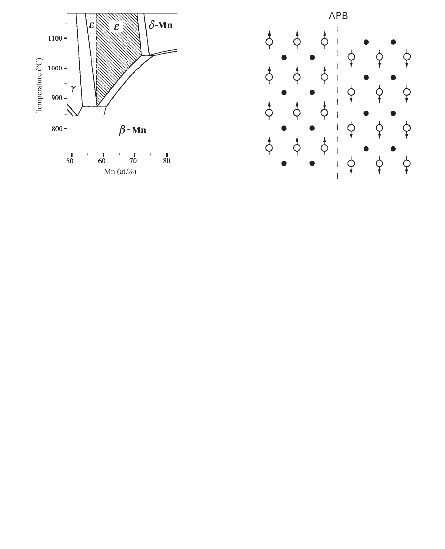
A second difﬁculty associated with MnAl alloys is

the metastable nature of the t-phase. In fact, this

phase is not found in the Mn–Al phase diagram (see

Fig. 2). It can be obtained by starting from the high-

temperature equilibrium e-phase occurring in this

concentration range, which has an h.c.p. structure.

However, the preparation of the f.c.t. t-phase from

the h.c.p. e-phase is not easy. Formerly it was be-

lieved that the t-phase forms from the e-phase via an

intermediate phase, e

, of orthorhombic structure

(B19) by means of the reaction scheme

h:c:p:ðeÞ-B19ðe

Þ-f:c:t:ðtÞ

where the h.c.p. structure (e) transforms ﬁrst into the

orthorhombic e

-phase by an atomic ordering reac-

tion. Subsequently, the metastable f.c.t. ferromagnetic

t-phase is formed by way of shear transformation.

However, this reaction scheme is rather unlikely in

480

Magnetic Materials: Hard

view of the observation by electron microscopy that

precipitates of the e

-phase in undercooled e do not act

as nucleation centers for t.

The occurrence of a massive transformation

has been proposed by Hoydick et al. (1997). It is

furthermore important to realize that the metastable

t-phase, after an annealing time that depends on

alloy composition and the annealing temperature,

tends to decompose into the two stable phases with

b-Mn (b) and Cr

type structure (g

). For this

reason, the annealing time has to be chosen carefully.

Various heat treatments have been proposed to

obtain and preserve the t-phase, as discussed in more

detail in the review of Mu

ller et al. (1996). In several

investigations (Otani et al. 1977, Pareti et al. 1986) it

has been shown that doping with carbon can lead to

significant improvements in the kinetics associated

with the formation and decomposition of the t-phase.

In the carbon-doped alloys, an incubation period

is involved with the formation of the t-phase. The

equilibrium phases b and g

do not form simultane-

ously with the t-phase, but form subsequently. The

upshot is that the retardation of the formation allows

for better process control because it also delays the

formation of the undesirable b- and g

-phases. Car-

bon doping has, furthermore, a beneﬁcial effect on

the saturation magnetization, although there is a

substantial decrease in Curie temperature.

The partial occupation of aluminum sites by man-

ganese atoms at (0,

) implies that many antiphase

domain boundaries occur in the crystal lattice of the

t-phase. As shown in Fig. 3, these antiphase domain

boundaries can act as nucleation sites for Bloch

walls, which leads to a relatively easy magnetization

reversal and hence to low values of the coercivity and

remanence.

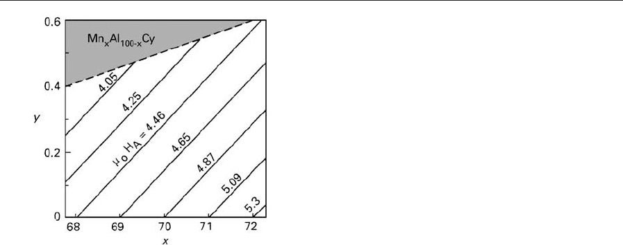
The magnetic properties of the t-phase in the con-

centration range 67–73 wt.% manganese have been

investigated by Pareti et al. (1986). It has been shown

that an increasing manganese concentration in the

homogeneity range of the t-phase leads to an increase

in the Curie temperature but it lowers the saturation

magnetization. The increase of T

is the result of a

general increase of the exchange interaction when

magnetic manganese replaces nonmagnetic alumi-

num. The decrease of the saturation magnetization

originates from the excess manganese atoms occupy-

ing former aluminum sites. These manganese mo-

ments, when coupled antiparallel to those of the main

lattice, can cause a reduction in the net saturation

moment. The anisotropy ﬁeld shows a slight increase

with manganese content. According to Pareti et al.

(1986) this increase in H

is not a real increase in

anisotropy but merely reﬂects the fact that the an-

isotropy constant, K

¼M

/2, remains approxi-

mately constant since M

decreases with manganese

concentration. The effect of carbon addition and al-

uminum concentration on the anisotropy ﬁeld is

shown in Fig. 4.

An important improvement in the magnet manu-

facturing is due to Otani et al. (1977). They have

shown that the hard magnetic properties can be sig-

nificantly enhanced when using a high-temperature

extrusion process. In this process microstructures are

realized consisting of very ﬁne grains while also the

number of antiphase boundaries is strongly reduced.

The manufacturing route involves the following steps.

The alloys (typically 70.0 wt.% Mn, 29.5 wt.% Al,

Figure 3

Schematic representation of an antiphase boundary and

the corresponding reversal in magnetization direction

across the boundary.

Figure 2

Central portion of the Mn–Al phase diagram as

reported by Liu et al. (1996). The shaded area of the

homogeneity region of the b-phase corresponds to alloys

that transform into b-Mn on quenching.

481

Magnetic Materials: Hard

0.5 wt.% C) are given a homogenizing treatment at

1100 1C for 1 h. After quenching the ingots to 500 1C

they are annealed at 600 1C for 30 min. The hot ex-

trusion is performed at 700 1C with a pressure of

80 kgmm

2

. Finally, the extruded material is aged at

700 1C for 10 min. The energy product can reach val-

ues close to 56 kJm

3

(7 MGOe). Compared with the

energy products reached in rare earth-based magnets

(see Rare Earth Magnets: Materials) these values are

very low. However, one has to take into consideration

that the raw materials costs are much lower. More-

over, the production cost is much lower because the

whole processing route can be performed in air.

See also: Ferrite Magnets: Improved Performance;

Hard Magnetic Materials, Basic Principles of

Bibliography

Buschow K H J 1997 Magnetism and processing of permanent

magnet materials. In: Buschow K H J (ed.) Handbook of

Magnetic Materials. Elsevier, Amsterdam, Vol. 10, Chap. 4

Hoydick D P, Palmiere E J, Soffa W A 1997 Microstructural

development in Mn–Al base permanent magnet materials:

new perspectives. J. Appl. Phys. 81, 5624–6

Kaneko H, Homma M, Suzuki K 1968 A new heat treatment of

Pt–Co alloys of high-grade magnetic properties. Trans. JIM

9, 124–9

Liu J P, Luo C P, Liu Y, Sellmyer D J 1998 High energy

products in rapidly annealed nanoscale Fe/Pt multilayers.

Appl. Phys. Lett. 72, 483–5

Liu X J, Kainuma R, Ohtani H, Ishida K 1996 Phase equilibria

in the Mn-rich portion of the binary system Mn–Al. J. Alloys

Compds. 235, 256–61

ller Ch, Stadelmaier H H, Reinsch B, Petzow G 1996 Met-

allurgy of the magnetic t-phase in Mn–Al and Mn–Al–C.

Z. Metallkd. 87, 594–7

Otani T, Kato N, Kojima S, Kojima K, Sakomoto Y, Konno I,

Tsukahara M, Kubo T 1977 Magnetic properties of Mn–

Al–C permanent magnets. IEEE Trans. Magn. MAG-13,

1328–30

Pareti L, Bolzoni F, Leccabue F, Ermakov A E 1986 Magnetic

anisotropy of MnAl and MnAlC permanent magnets.

J. Appl. Phys. 59, 3824–8

Tanaka Y, Kimura N, Hono K, Yasuda K, Sakurai T 1997

Microstructure and magnetic properties of Fe–Pt permanent

magnets. J. Magn. Magn. Mater. 170, 289–97

Watanabe K 1991 Permanent magnetic properties and their

temperature dependence in the Fe–Pt–Nb alloy system. Ma-

ter. Trans. JIM 32, 292–8

Zhang B, Soffa W A 1994 The structure and properties of L1

ordered ferromagnetic Co–Pt, Fe–Pt, Fe–Pd and Mn–Al.

Scr. Metall. 30, 683–8

K. H. J. Buschow

University of Amsterdam, The Netherlands

Magnetic Materials: Transmission

Electron Microscopy

The application potential of many advanced magnet-

ic materials depends on a combination of the intrinsic

and extrinsic properties of the materials in question.

Hence a detailed knowledge of both the physical and

magnetic microstructure is essential if the structure–

property relation is to be understood and materials

with optimized properties produced. Most of the ma-

terials of interest today are markedly inhomogeneous

with features requiring resolution on a sub-50 nm

scale for their detailed investigation. Transmission

electron microscopy (TEM) has two primary attrac-

tions. It offers very high spatial resolution and, be-

cause of the large number of interactions that take

place when a beam of fast electrons hits a thin solid

specimen, detailed insight into compositional, elec-

tronic, as well as structural and magnetic, properties.

The resolution that is achievable depends largely on

the information sought and may well be limited by

the specimen itself. Typical resolutions achievable for

structural imaging are 0.2–1.0 nm, for extraction of

compositional information 0.5–3.0 nm, and for mag-

netic imaging 2–20 nm.

Although TEM is used extensively for both micro-

structural and micromagnetic studies it is only the

latter that are considered in this chapter. It begins

with a description of the basic interaction, which al-

lows magnetic domains to be revealed. Thereafter a

Figure 4

Dependence of the room temperature anisotropy ﬁeld,

, on carbon and manganese content in Mn

100x

with 68oxo72wt.% and 0oyo0.6 wt.%. Constant

anisotropy ﬁeld values are represented by solid lines.

The shaded area corresponds to alloys above the carbon

solubility limit (after Pareti et al. 1986).

482

Magnetic Materials: Transmission Electron Microscopy

brief description is given of the most widely used im-

aging modes together with the performance expecta-

tion of each. Studies can be made of specimens in

their as-prepared states, in remanent states and in the

presence of applied ﬁelds. From these can be derived

basic micromagnetic information, the nature of do-

main walls, where nucleation occurs, and the impor-

tance or otherwise of domain wall pinning and many

other related phenomena. It is only recently that ex-

tensive in situ magnetizing experiments have been

undertaken and there is a short discussion of the

various ways of implementing them. In the ﬁnal sec-

tion, examples of the application of TEM to magnetic

materials are given. As TEM is essentially restricted

to viewing material sections o200 nm thick, it is ide-

ally suited to the study of thin ﬁlms. Illustrative ex-

amples for both hard and soft ﬁlms are presented.

However, useful information on bulk magnetic ma-

terial can also be determined and the use of TEM in

this area is discussed briefly.

1. Imaging Magnet ic Structures by TEM

The principal difﬁculty encountered when using a

TEM to study magnetic materials is that the lenses

are essentially electromagnets and the specimen is

usually immersed in the high magnetic ﬁeld (typi-

cally 40.6 T) of the objective lens. This is sufﬁcient

to completely eradicate or severely distort most do-

main structures of interest. A number of strategies

have been devised to overcome the problem of the

high ﬁeld in the specimen region (McFadyen and

Chapman 1992). These include (i) simply switching

off the standard objective lens, (ii) changing the

position of the specimen so that it is no longer im-

mersed in the objective lens ﬁeld, (iii) retaining the

specimen in its standard position but changing the

pole-pieces, once again to provide a non-immersion

environment, or (iv) adding super mini-lenses in ad-

dition to the standard objective lens which is once

again switched off. The last named is the preferred

option as it offers both high performance and min-

imum disruption to the other microscope functions.

Magnetic structures are most commonly revealed

in the TEM using one of the modes of Lorentz mi-

croscopy. This generic name is used to describe all

imaging modes in which contrast is generated as a

result of the deﬂection experienced by electrons as

they pass through a region of magnetic induction

(Hale et al. 1959). The Lorentz deﬂection angle b

given by

¼ eltðB  nÞ=h ð1Þ

where B is the induction averaged along an electron

trajectory, n is a unit vector parallel to the incident

beam, t is the specimen thickness, and l is the elec-

tron wavelength. Substituting typical values into Eqn.

(1) shows that b

rarely exceeds 100 mrad. Given the

small magnitude of b

there is no danger of confusing

magnetic scattering with the more familiar Bragg

scattering where angles are typically in the range

1–10 mrad.

The description given so far is classical and much

of Lorentz imaging can be understood in these terms.

However, for certain imaging modes and, more gen-

erally if a full quantitative description of the spatial

variation of induction is sought, a quantum mechan-

ical description of the beam-specimen interaction

must be sought (Aharanov and Bohm 1959). Using

this approach the magnetic ﬁlm should be considered

as a phase modulator of the incident electron wave,

the phase gradient =j of the specimen transmittance

being given by

=j ¼ 2petðB  nÞ=h ð2Þ

where e and h are the electronic charge and Planck’s

constant respectively. Substituting typical numerical

values shows that magnetic ﬁlms should normally be

regarded as strong, albeit slowly varying, phase ob-

jects. For example, the phase change involved in

crossing a domain wall usually exceeds p rad.

2. Imaging Modes in Lorentz Microscopy

Magnetic imaging can be performed in either ﬁxed-

beam or conventional (C)TEMs or in scanning

(S)TEMs. Examples of each along with their associ-

ated advantages and drawbacks are given below.

Fuller details on the techniques can be found in

Reimer (1984), Jakubovics (1994), Chapman (1984),

and Chapman and Scheinfein (1999).

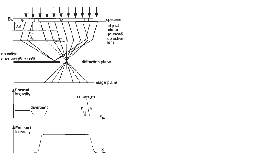
2.1 Fresnel and Foucault Imaging

The most commonly used techniques for revealing

magnetic domain structures are the Fresnel (or defo-

cus) and Foucault imaging modes. Both are normally

practiced in a CTEM. Schematics of how magnetic

contrast is generated are shown in Fig. 1. For the

purpose of illustration, a simple specimen comprising

three domains separated by two 1801 domain walls is

assumed. In Fresnel microscopy the imaging lens is

simply defocused so that the object plane is no longer

coincident with the specimen. Narrow dark and

bright bands, delineating the positions of the domain

walls, can then be seen in an otherwise contrast-free

image. For Foucault microscopy, a contrast-forming

aperture must be present in the plane of the diffrac-

tion pattern and this is used to obstruct one of the

two components into which the central diffraction

spot is split due to the deﬂections suffered as the

electrons pass through the specimen. Note that in

general, the splitting of the central spot is more com-

plex than for the simple case considered here. As a

result of the partial obstruction of the diffraction

483

Magnetic Materials: Transmission Electron Microscopy

spot, domain contrast can be seen in the image.

Bright areas correspond to domains where the mag-

netization orientation is such that electrons are de-

ﬂected through the aperture and dark areas to those

where the orientation of magnetization is oppositely

directed.

The principal advantages of Fresnel and Foucault

microscopy together are that they are fairly simple to

implement and they provide a clear picture of the

overall domain geometry and a useful indication of the

directions of magnetization in (at least) the larger

domains. Such attributes make them the preferred

techniques for in situ experimentation (see Sect. 3).

However, a significant drawback of the Fresnel mode

is that no information is directly available about the

direction of magnetization within any single domain,

whilst reproducible positioning of the contrast-

forming aperture in the Foucault mode is difﬁcult.

Moreover, both imaging modes suffer from the dis-

advantage that the relation between image contrast

and the spatial variation of magnetic induction is usu-

ally nonlinear. Thus extraction of reliable quantitative

data, especially from regions where the induction

varies rapidly, is problematic.

Part solutions to these problems have very recently

been provided. Whilst the statements made above

stand if a single Fresnel image is considered, a novel

development (proposed by Paganin and Nugent

(1998)) is to make use of two images of exactly the

same area recorded with the same values of under- and

over-focus. By combining the images in different ways

maps of the two orthogonal components of magnetic

induction perpendicular to the direction of electron

travel can be obtained. Initial results look very prom-

ising but it remains to be seen down to what level

reliable information can be extracted. A variant on

standard Foucault microscopy—coherent Foucault

imaging—has been introduced by Johnston and

Chapman (1995). Here the standard objective aper-

ture is replaced by a thin ﬁlm aperture, which instead

of obscuring part of the central diffraction spot simply

phase shifts those parts passing through the ﬁlm.

Provided there is a region of free space close to the

magnetic specimen and the thin ﬁlm aperture is po-

sitioned to cut the (undeﬂected) diffraction spot aris-

ing from the free space area, the image takes the form

of a magnetic interferogram corresponding to the

lines of ﬂux running through the magnetic specimen.

Similar interferograms are generated using electron

holography and further discussion is delayed until

Sect. 2.4.

2.2 Low Angle Diffraction

An alternative approach towards determining quan-

titative data from the TEM is by directly observing

the form of the split central diffraction spot. The

main requirement for low angle diffraction (LAD) is

that the magniﬁcation of the intermediate and pro-

jector lenses of the microscope is sufﬁcient to render

visible the small Lorentz deﬂections. Camera con-

stants (deﬁned as the ratio of the displacement of the

beam in the observation plane to the deﬂection angle

itself) in the range 30–100 m are typically required.

Furthermore, high spatial coherence in the illumina-

tion system is essential if the detailed form of the low

angle diffraction pattern is not to be obscured. In

practice this necessitates the angle subtended by the

illuminating radiation at the specimen to be consid-

erably smaller than the Lorentz angle of interest. The

latter condition is particularly easy to fulﬁl in a TEM

equipped with a ﬁeld emission gun (FEG). Thus

whilst LAD moves some way to supplementing the

deﬁciencies of standard Fresnel and Foucault imag-

ing, the fact that it provides global information from

the whole of the illuminated specimen area rather

than local information means that alternative imag-

ing techniques are still desirable.

2.3 Differential Phase Contrast Imaging

Differential phase contrast (DPC) microscopy

(Dekkers and de Lang 1974, Chapman et al. 1990)

overcomes many of the deﬁciencies of the imaging

modes discussed above. Its normal implementation

Figure 1

Schematic of magnetic contrast generation in the Fresnel

and Foucault imaging modes.

484

Magnetic Materials: Transmission Electron Microscopy

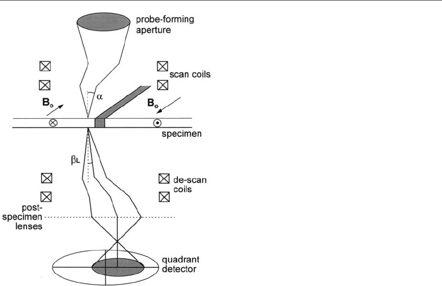
requires a STEM. It can usefully be thought of as

a local area LAD technique using a focused probe;

Fig. 2 shows a schematic of how contrast is generated.

In DPC imaging the local Lorentz deﬂection at the

position about which the probe is centered is deter-

mined using a segmented detector sited in the far

ﬁeld. Of specific interest are the difference signals from

opposite segments of a quadrant detector as these

provide a direct measure of the two components of b

By monitoring the difference signals as the probe is

scanned in a regular raster across the specimen, directly

quantiﬁable images with a resolution approximately

equal to the electron probe size are obtained. Providing

a FEG microsco pe is used, probe sizes o10 nm can be

achieved with the specimen located in ﬁeld-free space.

A full wave-optical analysis of the image formation

process conﬁrms the validity of the simple geometric

optics argument outlined above for experimentally re-

alizable conditions. The main disadvantage against

which this must be set is the undoubted increase in

instrumental complexity and operational difﬁculty

compared with the ﬁxed-beam imaging modes.

The two difference-signal images are collected si-

multaneously and are therefore in perfect registra-

tion. From them a map of the component of

magnetic induction perpendicular to the electron

beam can be constructed. In addition a third image

formed by the total signal falling on the detector can

be formed. Such an image contains no magnetic in-

formation (the latter being dependent only on vari-

ations in the position of the bright ﬁeld diffraction

disk in the detector plane) but is a standard incoher-

ent bright ﬁeld image as would be obtained using an

undivided spot detector. Thus a perfectly registered

structural image can be built up at the same time as

the two magnetic images, a further distinct advantage

of DPC imaging. However, at this point it is impor-

tant to recognize one of the primary difﬁculties en-

countered in all Lorentz microscopy modes. The

simple analyses given above have assumed that image

contrast arises solely as a result of the magnetic in-

duction/electron beam interaction whereas, in reality,

contrast arising from the physical microstructure is

present virtually always as well. Moreover, it is fre-

quently stronger than that of magnetic origin with the

result that the resolution at which useful magnetic

information is extracted is often limited by the spec-

imen rather than the inherent instrumental capability.

Although the presence of unwanted contrast of

structural origin is serious, its effect can be amelio-

rated to some extent by suitable choice of operating

conditions or modiﬁcation of the techniques them-

selves. It is frequently (but not always!) the case that

the physical microstructure is on a significantly

smaller scale than its magnetic counterpart. If this

is so, the inﬂuence of high spatial frequency compo-

nents in the image can be reduced by substitution of

the solid quadrant detector by its annular counter-

part (Chapman et al. 1990). Indeed, in the latter case,

not only is the unwanted signal component sup-

pressed considerably but the signal-to-noise ratio in

the magnetic component is significantly enhanced.

2.4 Electron Holography

Whilst DPC imaging can provide high spatial reso-

lution induction maps and direct information on do-

main wall structures, difﬁculties still remain when

absolute values of b

, rather than relative variations,

are sought. A ﬁnal class of techniques, involving

electron holography, go some way to overcoming this

problem. Here the electron wave, phase-shifted after

passing through the specimen in accordance with

Eqn. (2), is mixed with a reference wave and the re-

sulting interference pattern is analyzed to yield a full

quantitative description of the averaged induction

perpendicular to the electron trajectory. Several dis-

tinct strategies exist for mixing the specimen and ref-

erence waves and for realizing an interpretable image.

In off-axis holographic techniques, a charged wire

acts as a biprism, which is located before the spec-

imen in scanning TEMs (Mankos et al. 1994) and

after it in ﬁxed-beam instruments (Tonomura 1987,

Figure 2

Schematic of magnetic contrast generation in the DPC

imaging mode.

485

Magnetic Materials: Transmission Electron Microscopy

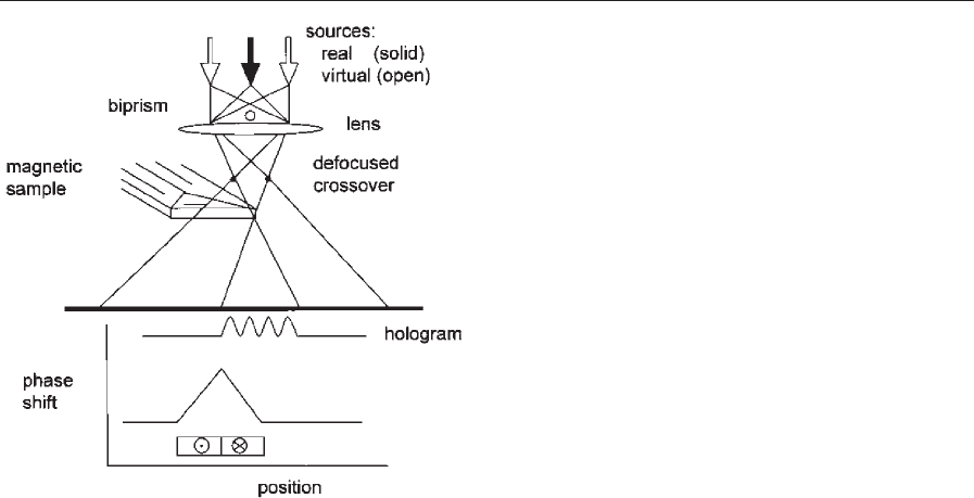
Dunin-Borkowski et al. 1998). Figure 3 shows a

schematic relating to the former case. Images gener-

ated by holography are frequently in the form of

magnetic interferograms which can be produced

directly or by computer- or optical-processing of

recorded holograms. The ﬂux enclosed between ad-

jacent fringes in the interferograms is h/e and so ab-

solute values of the induction integrated along an

electron trajectory can be determined. Difﬁculties

with holographic techniques are the high level of in-

strumental sophistication (a FEG is essential and

other instrumental modiﬁcations are usually manda-

tory), the difﬁculty of imaging away from specimen

edges where suitable reference beams are inaccessible,

the rapid deterioration in performance with increas-

ing inelastic scattering (severely restricting maximum

specimen thicknesses accessible) and excessive fringe

separations when very thin specimens are under in-

vestigation. Thus, whilst a very powerful addition to

the available techniques of Lorentz microscopy, ho-

lography brings with it its own associated problems

and limitations.

3. In Situ Studies of Magnetization Reversal

by TEM

One of the major attributes of TEM is the ability to

change the magnetic state of the specimen in situ.To

observe how magnetic structures evolve as a function

of temperature is particularly straightforward, and

simply involves mounting the specimen in a variable

temperature holder. The use of a small furnace built

into a holder allows temperatures to be raised

from room temperature to temperatures in excess of

1200 K, which is beyond the Curie temperature of

essentially all magnetic materials of interest. Alter-

natively, cooling holders can be used in which case

the temperatures attained depend on whether liquid

nitrogen or helium is the coolant employed. In these

cases, the minimum temperatures at the points of

observation are usually significantly greater than the

liquefaction temperatures of the coolants involved.

Realistic temperatures achievable at the center of a

thin ﬁlm specimen are 110 K and 20 K for liquid ni-

trogen and liquid helium respectively. Lower temper-

atures are difﬁcult to achieve mainly as a result of

poor thermal paths rather than because of significant

heating in the electron beam itself. The energy de-

posited, and hence the consequent temperature rise, is

generally very small in a thin ﬁlm sample.

For magnetic specimens, in situ observations of the

magnetization reversal process itself are crucial if, for

example, hysteresis is to be understood at a micro-

scopic level. There are two different approaches to

subjecting the specimen to varying magnetic ﬁelds in

a TEM. In the ﬁrst a magnetizing stage is used which

generates a horizontal ﬁeld in the plane of the

specimen. Two variants are possible. A magnetizing

stage can be built into the specimen mounting rod

(Hefferman et al. 1990) or, if spare ports are available

at appropriate positions in the microscope column,

one can be introduced as a separate entity. As the

maximum available ﬁeld relates strongly to the vol-

ume of the exciting coils and the nature of the mag-

netic circuit, greater ﬁelds can usually be generated

using an independent stage. However, irrespective of

which variation is adopted, the presence of a hori-

zontal ﬁeld over a vertical distance many times great-

er than the specimen thickness results in the electron

beam being deﬂected through an angle orders of

magnitude greater than typical Lorentz angles. Under

these conditions the illumination normally disappears

from the ﬁeld of view and can only be restored using

compensating coils. This introduces an additional el-

ement of complexity and the inevitable result is that

in such experiments there is limited opportunity to

observe changes as they occur; rather the changes

that took place due to a change of ﬁeld are normally

observed some time after the event.

An alternative approach, which can be used in in-

struments where super mini-lenses are present as well

as the standard objective lens, is to use the latter

as a source of magnetic ﬁeld given that the specimen

remains located somewhere close to its center

(Chapman et al. 1995, McVitie et al. 1995). The

objective lens now acts as a source of vertical ﬁeld

whose excitation is under the control of the experi-

menter. Variation in the excitation of the mini-lenses

compensates for the additional focusing effect

Figure 3

Schematic of how electron holography is implemented in

a scanning instrument.

486

Magnetic Materials: Transmission Electron Microscopy

introduced. As the ﬁeld of the objective lens is par-

allel to the optic axis, it is clearly suitable for studying

magnetization processes in perpendicular magnetic

materials. However, by tilting the specimen, a com-

ponent of ﬁeld in the plane of the specimen can also

be introduced. Furthermore, given that demagnetiz-

ing effects perpendicular to the plane of a thin ﬁlm

are very large, the presence of even moderately large

perpendicular ﬁelds can often be ignored and it is the

smaller ﬁelds in the plane of the specimen that are of

interest. When this is the case the objective is set to an

appropriate ﬁxed excitation giving a constant vertical

ﬁeld and the sample is simply tilted from a positive

angle to a negative one and back again to take it

through a magnetization cycle. The principal attrac-

tion of the second approach is that the electron op-

tical conditions do not vary during the experiment.

Hence, the specimen can be observed throughout and

the experimenter can devote full attention to the

changing magnetization distribution. It is this ap-

proach, which has been used primarily to obtain the

results described in the following section.

4. Illustrative Examples of the Use of TEM to

Study Soft and Hard Magnetic Materials

In this section the use of TEM is illustrated with ref-

erence to some materials systems of current magnetic

interest. Soft and hard magnetic ﬁlms, as well as dis-

playing many fascinating scientific properties are also

of major technological importance. Soft magnetic

ﬁlms are used extensively as sensors whilst hard mag-

netic ﬁlms are the material of choice for storing in-

formation in hard disks and other recording systems.

As an example of the former, some magnetic images

from spin-valves are presented (Sect. 4.1) whilst do-

main studies in thin CoPt ﬁlms serve to show the kind

of small-scale domain structure found in magnetically

hard ﬁlms (Sect. 4.2). TEM is also used to study bulk

materials such as hard magnetic alloys used in per-

manent magnets. However, unlike the case with thin

ﬁlms where specimen preparation is at most restricted

to the removal of an underlying substrate, here the

magnetic material itself must be thinned. Once thin-

ning is undertaken, particularly to the extent required

for TEM, the macroscopic magnetic properties them-

selves change markedly. Thus, taking sintered NdFeB

as an example, the grain size is likely to be in the

range of 5–10 mm so that the domain structure exist-

ing in such a grain situated in the bulk of the material

will be quite different from that in a 100 nm thick

section of the material as typically used in TEM. This

arises primarily as a consequence of the increased

importance of the magnetostatic contribution to the

total energy in the latter case. Hence extreme care

must be taken in making deductions from TEM do-

main images. Despite this, useful information can be

extracted on, for example, magnetic coupling across

grain boundaries. Typical results are presented in

Sect. 4.3.

4.1 Domain Structures in Spin-valves

Reduced to its simplest form a spin-valve comprises

four thin layers (Dieny 1994, Kools 1996). Two are

ferromagnetic ﬁlms, frequently permalloy, which are

separated by a thin non-magnetic spacer, usually

copper. On top of one of the ferromagnetic layers is

deposited an antiferromagnetic ﬁlm, which serves to

‘‘pin’’ the magnetization of that layer. Changes in

resistance occur when the magnetization orientation

of the other magnetic layer—the so-called ‘‘free’’

layer—changes under the inﬂuence of a small mag-

netic ﬁeld. In the absence of any applied ﬁeld the

orientation of the free layer magnetization is gener-

ally parallel to that in the pinned layer due to weak

magnetostatic coupling between the layers. A mag-

netic ﬁeld of 5–30 Oe is often all that is required to

completely reverse the magnetization in the free layer.

Under such small ﬁelds there is no change in the ori-

entation of the pinned layer magnetization. To over-

come the exchange-biasing between the pinned layer

and the antiferromagnet and so effect a reversal of

the magnetization here, ﬁelds well in excess of 100 Oe

are the norm. For optimized sensor performance it is

important to know the mechanism by which each of

the two layers reverses and it is here that Lorentz

microscopy has a very important role to play.

Figure 4 shows Fresnel images of a spin-valve tak-

en under different applied ﬁelds. Initially both layers

are uniformly magnetized and no contrast is seen

(Fig. 4(a)). As the ﬁeld increases, magnetization

ripple becomes apparent (Fig. 4(b)) after which a

number of domain walls appear (Figs. 4(c, d)) and it

is clear that reversal is by domain propagation. The

walls are not particularly straight nor are they as

mobile as in a single isolated ferromagnetic permalloy

layer (Gillies et al. 1995). Another feature to notice is

that black-white walls form and these can be iden-

tiﬁed as 3601 structures (Figs. 4(e, f )); these have an

enhanced stability and do not disappear at the same

ﬁeld as the other walls. Once they have been anni-

hilated the reversal of the free layer is complete and

no further contrast changes are seen until much high-

er ﬁelds are applied. If information on the nature of

the walls themselves is required, the DPC mode is

appropriate. Figure 5 shows an image pair, sensitive

to orthogonal in-plane induction components, from

some 3601 walls formed during the reversal of the free

layer. These images, recorded at much higher mag-

niﬁcation give direct information of the proﬁle of this

complex domain structure.

At higher ﬁelds magnetic contrast again appears as

the reversal of the pinned layer commences. Figure 6

shows examples of the kind of domain structure that

occurs in pinned or exchange-biased layers. The most

487

Magnetic Materials: Transmission Electron Microscopy

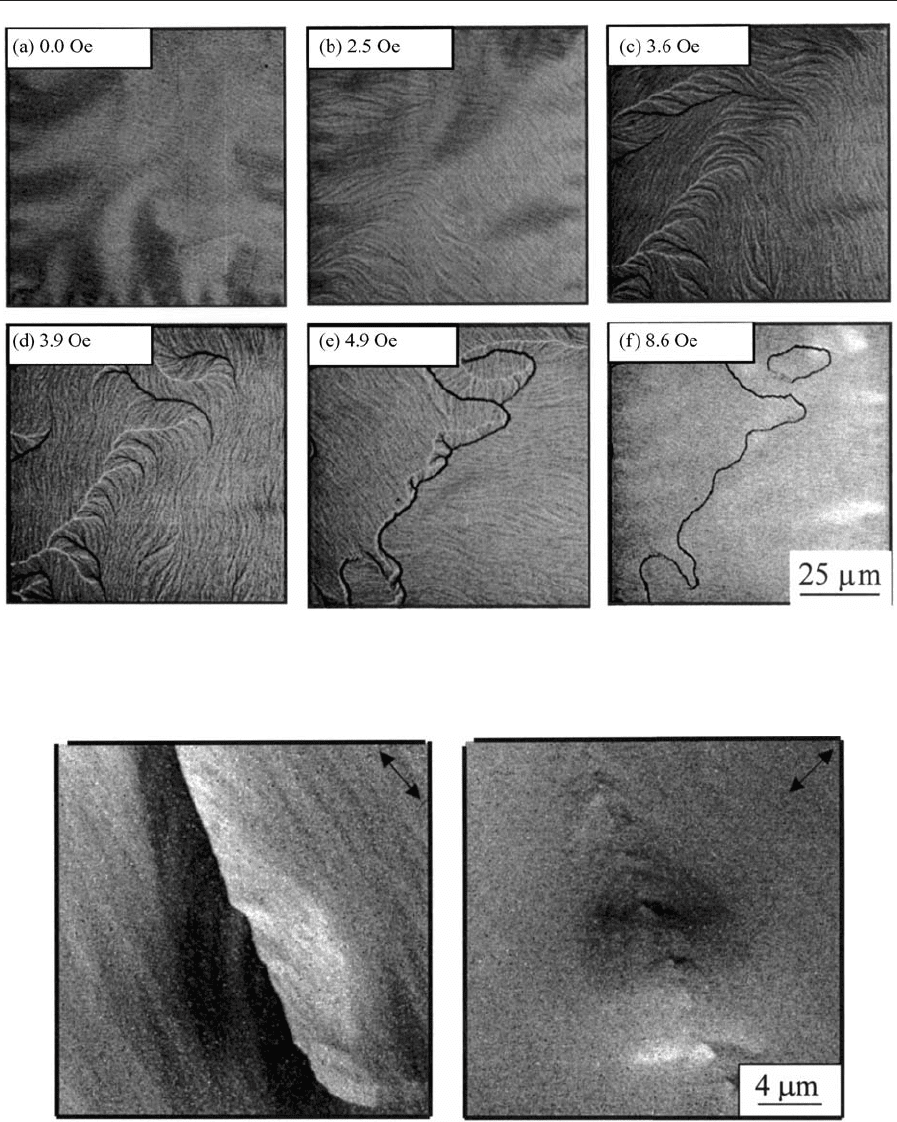
Figure 4

(a)–(f) Fresnel image sequence showing magnetization reversal of the free layer in a spin-valve. Fields at which each

image was recorded are shown in the insets.

Figure 5

DPC images of a 3601 wall segment in the free layer of a spin-valve. The arrows denote the direction of induction

mapped in each image.

488

Magnetic Materials: Transmission Electron Microscopy

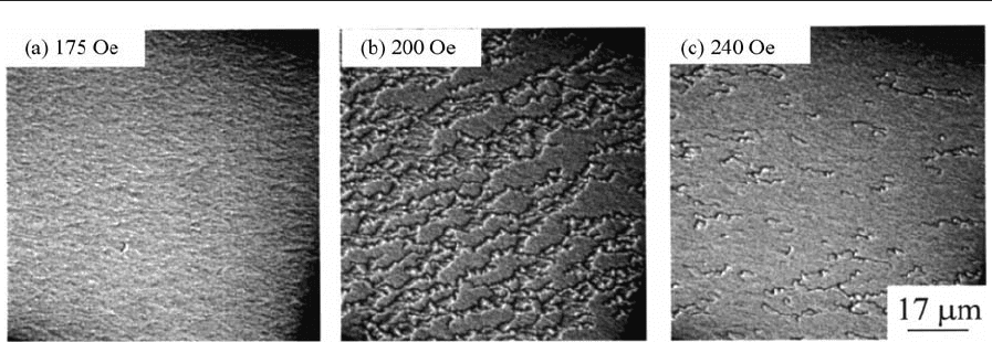
important point to note is that whilst reversal is again

primarily by domain processes, the geometry and

scale of the resulting domains are completely differ-

ent from those observed in the free layer.

4.2 Domain Structures in CoPt Films with in-plane

Magnetization

The storage layer in a hard disk is almost universally

a thin ﬁlm with a granular structure (Richter 1999).

Most usually the main constituent is cobalt but up to

four additional elements can be present in commer-

cial hard disk media, the most important additions

being chromium and/or platinum. The ﬁlms them-

selves are generally produced by sputtering and have

a mean grain size in the 10–15 nm range. The roles of

the additional elements are to achieve very small

grains with a tight size distribution and to reduce

substantially the exchange coupling between individ-

ual grains. The latter is of the utmost importance if

the medium is to support small domains and this, in

turn, is necessary if information is to be stored at high

density. If the medium does not support small do-

mains, or if the stability of these domains is low, then

the bit pattern, written by the recording head, chang-

es with consequent loss of information. To avoid ac-

cidental erasure and to minimize the effect of thermal

demagnetization, the coercivity of the cobalt alloys

must be high. Hence, if Lorentz microscopy is to be

used effectively to study domain processes in hard

cobalt alloy ﬁlms it is necessary to be able to subject

the specimen to changing ﬁelds in the range 1–3 kOe.

Whilst observation in these ﬁelds may also be desir-

able, it is frequently not necessary as it is irreversible

changes in the magnetization distribution that are of

the greatest interest here. Hence observations can be

made, for example, of a remanence as opposed to a

hysteresis cycle. Figure 7 shows Foucault images and

their associated LAD patterns at different stages in a

remanence cycle. Fresnel imaging is not appropriate

here as the wall contrast simply does not stand out

against the relatively high crystallographic contrast

present. From the Foucault images, it is clear that the

ﬁlm does support small domains (linear dimensions

of the smallest domains p100 nm); from the LAD

patterns, the overall dispersion of the magnetization

in the corresponding states can be assessed from the

variation in circumferential intensity around the arcs.

4.3 Domain Structures in Thin Sections of

NdFeB-type Alloys

As noted in the introduction to this section, the infor-

mation obtainable from bulk specimens using Lorentz

microscopy is more limited than that from magnetic

thin ﬁlms. Nonetheless much useful information can

be gleaned and this is illustrated by reference to studies

on NdFeB-type alloys. These alloys are used exten-

sively as high-energy product permanent magnets and

derive their attractive properties from a combination

of intrinsic and extrinsic properties, the latter depend-

ing on the processing to which the materials are sub-

jected (Gutﬂeisch and Harris 1996, Buschow 1998).

TEM is thus needed to characterise both the physical

and magnetic microstructures although it is only the

latter, which is of interest here. At comparatively low

magniﬁcations and in an unmagnetized specimen,

Foucault imaging reveals the domain geometry and

allows the orientation of the magnetization in the do-

mains to be determined. Mismatches between orientat-

ions in nearby grains relate to the overall anisotropy

or lack of it in the sample. Furthermore, in some in-

stances estimates can be made of the domain wall

energy from studies of wall spacings in grains whose

Figure 6

(a)–(c) Fresnel image sequence showing magnetization reversal of an exchange-biased layer. Fields at which each

image was recorded are shown in the insets.

489

Magnetic Materials: Transmission Electron Microscopy