Brealey, Myers. Principles of Corporate Finance. 7th edition

Brealey−Meyers:

Principles of Corporate

Finance, Seventh Edition

II. Risk 8. Risk and Return

Companies, 2003

2. If the investor can lend or borrow at the risk-free rate of interest, one

efficient portfolio is better than all the others: the portfolio that offers the

highest ratio of risk premium to standard deviation (that is, portfolio S in

Figure 8.6). A risk-averse investor will put part of his money in this efficient

portfolio and part in the risk-free asset. A risk-tolerant investor may put all

her money in this portfolio or she may borrow and put in even more.

3. The composition of this best efficient portfolio depends on the investor’s

assessments of expected returns, standard deviations, and correlations. But

suppose everybody has the same information and the same assessments. If

there is no superior information, each investor should hold the same

portfolio as everybody else; in other words, everyone should hold the

market portfolio.

Now let’s go back to the risk of individual stocks:

4. Don’t look at the risk of a stock in isolation but at its contribution to

portfolio risk. This contribution depends on the stock’s sensitivity to

changes in the value of the portfolio.

5. A stock’s sensitivity to changes in the value of the market portfolio is known

as beta. Beta, therefore, measures the marginal contribution of a stock to the

risk of the market portfolio.

Now if everyone holds the market portfolio, and if beta measures each security’s

contribution to the market portfolio risk, then it’s no surprise that the risk premium

demanded by investors is proportional to beta. That’s what the CAPM says.

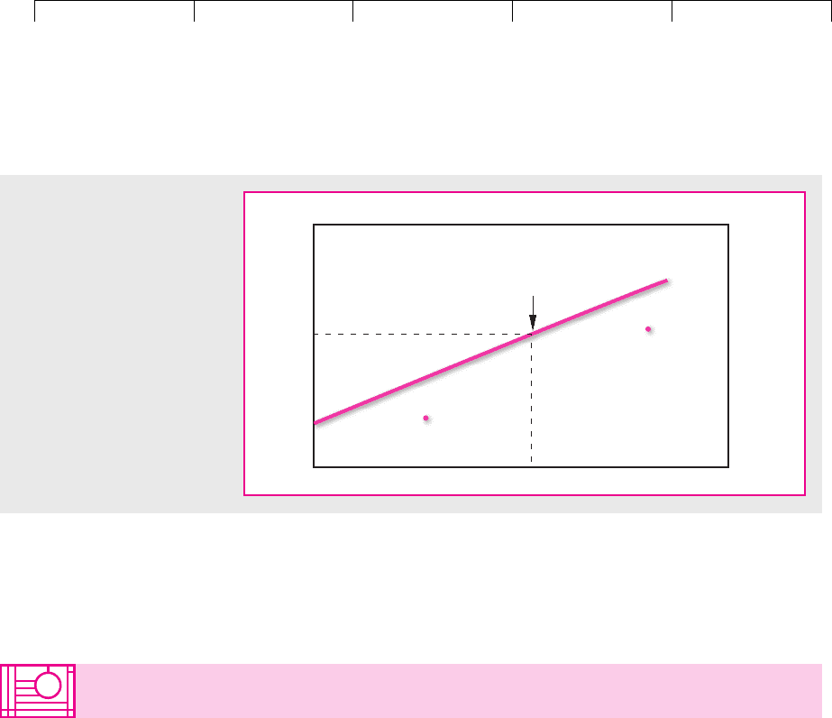
What If a Stock Did Not Lie on the Security Market Line?

Imagine that you encounter stock A in Figure 8.8. Would you buy it? We hope

not

—if you want an investment with a beta of .5, you could get a higher ex-

pected return by investing half your money in Treasury bills and half in the

market portfolio. If everybody shares your view of the stock’s prospects, the

price of A will have to fall until the expected return matches what you could get

elsewhere.

What about stock B in Figure 8.8? Would you be tempted by its high return?

You wouldn’t if you were smart. You could get a higher expected return for the

same beta by borrowing 50 cents for every dollar of your own money and invest-

ing in the market portfolio. Again, if everybody agrees with your assessment, the

price of stock B cannot hold. It will have to fall until the expected return on B is

equal to the expected return on the combination of borrowing and investment in

the market portfolio.

We have made our point. An investor can always obtain an expected risk pre-

mium of ␤(r

⫺ r

) by holding a mixture of the market portfolio and a risk-free loan.

So in well-functioning markets nobody will hold a stock that offers an expected

risk premium of less than ␤(r

⫺ r

). But what about the other possibility? Are there

stocks that offer a higher expected risk premium? In other words, are there any that

lie above the security market line in Figure 8.8? If we take all stocks together, we

have the market portfolio. Therefore, we know that stocks on average lie on the line.

Since none lies below the line, then there also can’t be any that lie above the line. Thus

CHAPTER 8

Risk and Return 197

Unless, of course, we were trying to sell it.

Brealey−Meyers:

Principles of Corporate

Finance, Seventh Edition

II. Risk 8. Risk and Return

Companies, 2003

each and every stock must lie on the security market line and offer an expected risk

premium of

r ⫺ r

⫽␤1r

⫺ r

198 PART II

Risk

Market

portfolio

Security

market line

1.51.0.50

Expected return

beta ( )

Stock B

Stock A

FIGURE 8.8

In equilibrium no stock can lie

below the security market line.

For example, instead of buying

stock A, investors would prefer

to lend part of their money and

put the balance in the market

portfolio. And instead of buying

stock B, they would prefer to

borrow and invest in the market

portfolio.

8.3 VALIDITY AND ROLE OF THE CAPITAL

ASSET PRICING MODEL

Any economic model is a simplified statement of reality. We need to simplify in or-

der to interpret what is going on around us. But we also need to know how much

faith we can place in our model.

Let us begin with some matters about which there is broad agreement. First, few

people quarrel with the idea that investors require some extra return for taking on

risk. That is why common stocks have given on average a higher return than U.S.

Treasury bills. Who would want to invest in risky common stocks if they offered only

the same expected return as bills? We wouldn’t, and we suspect you wouldn’t either.

Second, investors do appear to be concerned principally with those risks that

they cannot eliminate by diversification. If this were not so, we should find that

stock prices increase whenever two companies merge to spread their risks. And we

should find that investment companies which invest in the shares of other firms

are more highly valued than the shares they hold. But we don’t observe either phe-

nomenon. Mergers undertaken just to spread risk don’t increase stock prices, and

investment companies are no more highly valued than the stocks they hold.

The capital asset pricing model captures these ideas in a simple way. That is why

many financial managers find it the most convenient tool for coming to grips with

the slippery notion of risk. And it is why economists often use the capital asset pric-

ing model to demonstrate important ideas in finance even when there are other

ways to prove these ideas. But that doesn’t mean that the capital asset pricing

model is ultimate truth. We will see later that it has several unsatisfactory features,

and we will look at some alternative theories. Nobody knows whether one of these

alternative theories is eventually going to come out on top or whether there are

other, better models of risk and return that have not yet seen the light of day.

Brealey−Meyers:

Principles of Corporate

Finance, Seventh Edition

II. Risk 8. Risk and Return

Companies, 2003

Tests of the Capital Asset Pricing Model

Imagine that in 1931 ten investors gathered together in a Wall Street bar to discuss

their portfolios. Each agreed to follow a different investment strategy. Investor 1 opted

to buy the 10 percent of New York Stock Exchange stocks with the lowest estimated

betas; investor 2 chose the 10 percent with the next-lowest betas; and so on, up to in-

vestor 10, who agreed to buy the stocks with the highest betas. They also undertook

that at the end of every year they would reestimate the betas of all NYSE stocks and

reconstitute their portfolios.

Finally, they promised that they would return 60 years

later to compare results, and so they parted with much cordiality and good wishes.

In 1991 the same 10 investors, now much older and wealthier, met again in the

same bar. Figure 8.9 shows how they had fared. Investor 1’s portfolio turned out to

be much less risky than the market; its beta was only .49. However, investor 1 also

realized the lowest return, 9 percent above the risk-free rate of interest. At the other

extreme, the beta of investor 10’s portfolio was 1.52, about three times that of in-

vestor 1’s portfolio. But investor 10 was rewarded with the highest return, averag-

ing 17 percent a year above the interest rate. So over this 60-year period returns did

indeed increase with beta.

As you can see from Figure 8.9, the market portfolio over the same 60-year pe-

riod provided an average return of 14 percent above the interest rate

and (of

CHAPTER 8

Risk and Return 199

Betas were estimated using returns over the previous 60 months.

In Figure 8.9 the stocks in the “market portfolio” are weighted equally. Since the stocks of small firms

have provided higher average returns than those of large firms, the risk premium on an equally

weighted index is higher than on a value-weighted index. This is one reason for the difference between

the 14 percent market risk premium in Figure 8.9 and the 9.1 percent premium reported in Table 7.1.

.4 .6

Portfolio

beta

.8 1.0 1.2.2

1.4 1.6

Average risk premium,

1931–1991, percent

Investor 1

Investor 10

Market

portfolio

Market

line

FIGURE 8.9

The capital asset pricing model states that the expected risk premium from any investment

should lie on the market line. The dots show the actual average risk premiums from portfo-

lios with different betas. The high-beta portfolios generated higher average returns, just as

predicted by the CAPM. But the high-beta portfolios plotted below the market line, and four

of the five low-beta portfolios plotted above. A line fitted to the 10 portfolio returns would

be “flatter” than the market line.

Source: F. Black, “Beta and Return,” Journal of Portfolio Management 20 (Fall 1993), pp. 8–18.

Brealey−Meyers:

Principles of Corporate

Finance, Seventh Edition

II. Risk 8. Risk and Return

Companies, 2003

course) had a beta of 1.0. The CAPM predicts that the risk premium should increase

in proportion to beta, so that the returns of each portfolio should lie on the upward-

sloping security market line in Figure 8.9. Since the market provided a risk pre-

mium of 14 percent, investor 1’s portfolio, with a beta of .49, should have provided

a risk premium of a shade under 7 percent and investor 10’s portfolio, with a beta

of 1.52, should have given a premium of a shade over 21 percent. You can see that,

while high-beta stocks performed better than low-beta stocks, the difference was

not as great as the CAPM predicts.

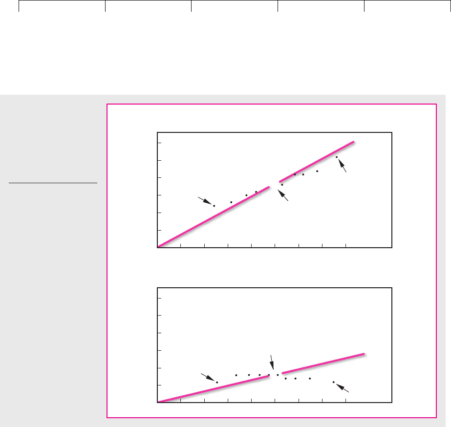
Although Figure 8.9 provides broad support for the CAPM, critics have

pointed out that the slope of the line has been particularly flat in recent years. For

example, Figure 8.10 shows how our 10 investors fared between 1966 and 1991.

Now it’s less clear who is buying the drinks: The portfolios of investors 1 and 10

had very different betas but both earned the same average return over these 25

years. Of course, the line was correspondingly steeper before 1966. This is also

shown in Figure 8.10

What’s going on here? It is hard to say. Defenders of the capital asset pricing

model emphasize that it is concerned with expected returns, whereas we can ob-

serve only actual returns. Actual stock returns reflect expectations, but they also

embody lots of “noise”—the steady flow of surprises that conceal whether on av-

200 PART II

Risk

.4 .6

Portfolio

beta

.8 1.0 1.2.2

1.4 1.6

Average risk premium,

1931–1965, percent

Investor 1

Investor 10

Market

portfolio

Market

line

.4 .6

Portfolio

beta

.8 1.0 1.2.2

1.4 1.6

Average risk premium,

1966–1991, percent

Investor 1

Investor 10

Market

portfolio

Market

line

3 4

7 8 9

FIGURE 8.10

The relationship

between beta and actual

average return has been

much weaker since the

mid-1960s. Compare

Figure 8.9.

Source: F. Black, “Beta and

Return,” Journal of Portfolio

Management 20 (Fall 1993),

pp. 8–18.

Brealey−Meyers:

Principles of Corporate

Finance, Seventh Edition

II. Risk 8. Risk and Return

Companies, 2003

erage investors have received the returns they expected. This noise may make it

impossible to judge whether the model holds better in one period than another.

Perhaps the best that we can do is to focus on the longest period for which there is

reasonable data. This would take us back to Figure 8.9, which suggests that ex-

pected returns do indeed increase with beta, though less rapidly than the simple

version of the CAPM predicts.

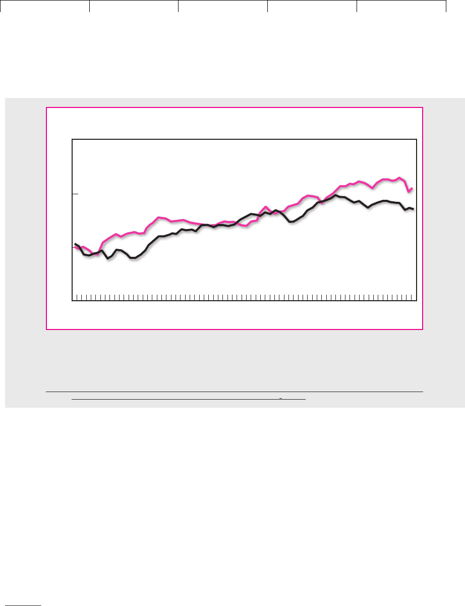
The CAPM has also come under fire on a second front: Although return has not

risen with beta in recent years, it has been related to other measures. For example,

the burgundy line in Figure 8.11 shows the cumulative difference between the re-

turns on small-firm stocks and large-firm stocks. If you had bought the shares with

the smallest market capitalizations and sold those with the largest capitalizations,

this is how your wealth would have changed. You can see that small-cap stocks did

not always do well, but over the long haul their owners have made substantially

CHAPTER 8

Risk and Return 201

A second problem with testing the model is that the market portfolio should contain all risky invest-

ments, including stocks, bonds, commodities, real estate—even human capital. Most market indexes

contain only a sample of common stocks. See, for example, R. Roll, “A Critique of the Asset Pricing The-

ory’s Tests; Part 1: On Past and Potential Testability of the Theory,” Journal of Financial Economics 4

(March 1977), pp. 129–176.

We say “simple version” because Fischer Black has shown that if there are borrowing restrictions,

there should still exist a positive relationship between expected return and beta, but the security mar-

ket line would be less steep as a result. See F. Black, “Capital Market Equilibrium with Restricted Bor-

rowing,” Journal of Business 45 (July 1972), pp. 444–455.

1932 1937 1942 1947 1952 1957 1962 1967 1972 1977 1982 1987 1992 1997

Year

0.1

100

Dollars

(log scale)

High minus low book-to-market

Small minus large

FIGURE 8.11

The burgundy line shows the cumulative difference between the returns on small-firm and large-firm

stocks. The blue line shows the cumulative difference between the returns on high book-to-market-

value stocks and low book-to-market-value stocks.

Source: www.mba.tuck.dartmouth.edu/pages/faculty/ken.french/data

library.

Brealey−Meyers:

Principles of Corporate

Finance, Seventh Edition

II. Risk 8. Risk and Return

Companies, 2003

higher returns. Since 1928 the average annual difference between the returns on the

two groups of stocks has been 3.1 percent.

Now look at the blue line in Figure 8.11 which shows the cumulative difference

between the returns on value stocks and growth stocks. Value stocks here are de-

fined as those with high ratios of book value to market value. Growth stocks are

those with low ratios of book to market. Notice that value stocks have provided a

higher long-run return than growth stocks.

Since 1928 the average annual differ-

ence between the returns on value and growth stocks has been 4.4 percent.

Figure 8.11 does not fit well with the CAPM, which predicts that beta is the only

reason that expected returns differ. It seems that investors saw risks in “small-cap”

stocks and value stocks that were not captured by beta.

Take value stocks, for ex-

ample. Many of these stocks sold below book value because the firms were in se-

rious trouble; if the economy slowed unexpectedly, the firms might have collapsed

altogether. Therefore, investors, whose jobs could also be on the line in a recession,

may have regarded these stocks as particularly risky and demanded compensation

in the form of higher expected returns.

If that were the case, the simple version

of the CAPM cannot be the whole truth.

Again, it is hard to judge how seriously the CAPM is damaged by this finding.

The relationship among stock returns and firm size and book-to-market ratio has

been well documented. However, if you look long and hard at past returns, you are

bound to find some strategy that just by chance would have worked in the past.

This practice is known as “data-mining” or “data snooping.” Maybe the size and

book-to-market effects are simply chance results that stem from data snooping. If

so, they should have vanished once they were discovered. There is some evidence

that this is the case. If you look again at Figure 8.11, you will see that in recent years

small-firm stocks and value stocks have underperformed just about as often as

they have overperformed.

There is no doubt that the evidence on the CAPM is less convincing than schol-

ars once thought. But it will be hard to reject the CAPM beyond all reasonable

doubt. Since data and statistics are unlikely to give final answers, the plausibility

of the CAPM theory will have to be weighed along with the empirical “facts.”

Assumptions behind the Capital Asset Pricing Model

The capital asset pricing model rests on several assumptions that we did not fully

spell out. For example, we assumed that investment in U.S. Treasury bills is risk-

free. It is true that there is little chance of default, but they don’t guarantee a real

202 PART II

Risk

The small-firm effect was first documented by Rolf Banz in 1981. See R. Banz, “The Relationship be-

tween Return and Market Values of Common Stock,” Journal of Financial Economics 9 (March 1981),

pp. 3–18. Fama and French calculated the returns on portfolios designed to take advantage of the size

effect and the book-to-market effect. See E. F. Fama and K. R. French, “The Cross-Section of Expected

Stock Returns,” Journal of Financial Economics 47 (June 1992), pp. 427–465. When calculating the returns

on these portfolios, Fama and French control for differences in firm size when comparing stocks with

low and high book-to-market ratios. Similarly, they control for differences in the book-to-market ratio

when comparing small- and large-firm stocks. For details of the methodology and updated returns on

the size and book-to-market factors see Kenneth French’s website (www

.mba.tuck.dartmouth.edu/

pages/faculty/ken.french/data library).

Small-firm stocks have higher betas, but the difference in betas is not sufficient to explain the differ-

ence in returns. There is no simple relationship between book-to-market ratios and beta.

For a good review of the evidence on the CAPM, see J. H. Cochrane, “New Facts in Finance,” Journal

of Economic Perspectives 23 (1999), pp. 36–58.

Brealey−Meyers:

Principles of Corporate

Finance, Seventh Edition

II. Risk 8. Risk and Return

Companies, 2003

return. There is still some uncertainty about inflation. Another assumption was

that investors can borrow money at the same rate of interest at which they can lend.

Generally borrowing rates are higher than lending rates.

It turns out that many of these assumptions are not crucial, and with a little

pushing and pulling it is possible to modify the capital asset pricing model to han-

dle them. The really important idea is that investors are content to invest their

money in a limited number of benchmark portfolios. (In the basic CAPM these

benchmarks are Treasury bills and the market portfolio.)

In these modified CAPMs expected return still depends on market risk, but the

definition of market risk depends on the nature of the benchmark portfolios.

practice, none of these alternative capital asset pricing models is as widely used as

the standard version.

CHAPTER 8

Risk and Return 203

For example, see M. C. Jensen (ed.), Studies in the Theory of Capital Markets, Frederick A. Praeger, Inc.,

New York, 1972. In the introduction Jensen provides a very useful summary of some of these variations

on the capital asset pricing model.

8.4 SOME ALTERNATIVE THEORIES

Consumption Betas versus Market Betas

The capital asset pricing model pictures investors as solely concerned with the

level and uncertainty of their future wealth. But for most people wealth is not an

end in itself. What good is wealth if you can’t spend it? People invest now to pro-

vide future consumption for themselves or for their families and heirs. The most

important risks are those that might force a cutback of future consumption.

Douglas Breeden has developed a model in which a security’s risk is measured

by its sensitivity to changes in investors’ consumption. If he is right, a stock’s ex-

pected return should move in line with its consumption beta rather than its market

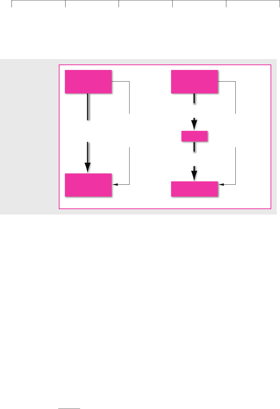
beta. Figure 8.12 summarizes the chief differences between the standard and con-

sumption CAPMs. In the standard model investors are concerned exclusively with

the amount and uncertainty of their future wealth. Each investor’s wealth ends up

perfectly correlated with the return on the market portfolio; the demand for stocks

and other risky assets is thus determined by their market risk. The deeper motive

for investing—to provide for consumption—is outside the model.

In the consumption CAPM, uncertainty about stock returns is connected di-

rectly to uncertainty about consumption. Of course, consumption depends on

wealth (portfolio value), but wealth does not appear explicitly in the model.

The consumption CAPM has several appealing features. For example, you don’t

have to identify the market or any other benchmark portfolio. You don’t have to

worry that Standard and Poor’s Composite Index doesn’t track returns on bonds,

commodities, and real estate.

However, you do have to be able to measure consumption. Quick: How much

did you consume last month? It’s easy to count the hamburgers and movie tick-

ets, but what about the depreciation on your car or washing machine or the daily

cost of your homeowner’s insurance policy? We suspect that your estimate of to-

tal consumption will rest on rough or arbitrary allocations and assumptions. And

if it’s hard for you to put a dollar value on your total consumption, think of the

Brealey−Meyers:

Principles of Corporate

Finance, Seventh Edition

II. Risk 8. Risk and Return

Companies, 2003

task facing a government statistician asked to estimate month-by-month con-

sumption for all of us.

Compared to stock prices, estimated aggregate consumption changes smoothly

and gradually over time. Changes in consumption often seem to be out of phase

with the stock market. Individual stocks seem to have low or erratic consumption

betas. Moreover, the volatility of consumption appears too low to explain the past

average rates of return on common stocks unless one assumes unreasonably high

investor risk aversion.

These problems may reflect our poor measures of con-

sumption or perhaps poor models of how individuals distribute consumption over

time. It seems too early for the consumption CAPM to see practical use.

Arbitrage Pricing Theory

The capital asset pricing theory begins with an analysis of how investors construct

efficient portfolios. Stephen Ross’s arbitrage pricing theory, or APT, comes from a

different family entirely. It does not ask which portfolios are efficient. Instead, it starts

by assuming that each stock’s return depends partly on pervasive macroeconomic in-

fluences or “factors” and partly on “noise”—events that are unique to that company.

Moreover, the return is assumed to obey the following simple relationship:

The theory doesn’t say what the factors are: There could be an oil price factor, an

interest-rate factor, and so on. The return on the market portfolio might serve as one

factor, but then again it might not.

Return ⫽ a ⫹ b

factor 1

2⫹ b

factor 2

2⫹ b

factor 3

2⫹

…

⫹ noise

204 PART II Risk

Wealth = market

portfolio

Market risk

makes wealth

uncertain.

Standard CAPM assumes

investors are concerned

with the amount and

uncertainty of future

wealth.

Consumption

Wealth is

uncertain.

Consumption is

uncertain.

Consumption CAPM

connects uncertainty

about stock returns

directly to uncertainty

about consumption.

(

)(

)

Stocks

(and other

risky assets)

Wealth

Stocks

(and other

risky assets)

FIGURE 8.12

(a) The standard

CAPM concentrates

on how stocks

contribute to the

level and uncertainty

of investor’s wealth.

Consumption is

outside the model.

(b) The consumption

CAPM defines risk as

a stock’s contribution

to uncertainty about

consumption. Wealth

(the intermediate

step between stock

returns and

consumption) drops

out of the model.

See R. Mehra and E. C. Prescott, “The Equity Risk Premium: A Puzzle,” Journal of Monetary Economics

15 (1985), pp. 145–161.

Brealey−Meyers:

Principles of Corporate

Finance, Seventh Edition

II. Risk 8. Risk and Return

Companies, 2003

Some stocks will be more sensitive to a particular factor than other stocks. Exxon

Mobil would be more sensitive to an oil factor than, say, Coca-Cola. If factor 1 picks

up unexpected changes in oil prices, b

will be higher for Exxon Mobil.

For any individual stock there are two sources of risk. First is the risk that stems

from the pervasive macroeconomic factors which cannot be eliminated by diversifi-

cation. Second is the risk arising from possible events that are unique to the company.

Diversification does eliminate unique risk, and diversified investors can therefore ig-

nore it when deciding whether to buy or sell a stock. The expected risk premium on

a stock is affected by factor or macroeconomic risk; it is not affected by unique risk.

Arbitrage pricing theory states that the expected risk premium on a stock should

depend on the expected risk premium associated with each factor and the stock’s

sensitivity to each of the factors (b

, b

, etc.). Thus the formula is

Notice that this formula makes two statements:

1. If you plug in a value of zero for each of the b’s in the formula, the

expected risk premium is zero. A diversified portfolio that is constructed

to have zero sensitivity to each macroeconomic factor is essentially risk-

free and therefore must be priced to offer the risk-free rate of interest. If

the portfolio offered a higher return, investors could make a risk-free (or

“arbitrage”) profit by borrowing to buy the portfolio. If it offered a lower

return, you could make an arbitrage profit by running the strategy in

reverse; in other words, you would sell the diversified zero-sensitivity

portfolio and invest the proceeds in U.S. Treasury bills.

2. A diversified portfolio that is constructed to have exposure to, say, factor 1,

will offer a risk premium, which will vary in direct proportion to the

portfolio’s sensitivity to that factor. For example, imagine that you construct

two portfolios, A and B, which are affected only by factor 1. If portfolio A is

twice as sensitive to factor 1 as portfolio B, portfolio A must offer twice the

risk premium. Therefore, if you divided your money equally between U.S.

Treasury bills and portfolio A, your combined portfolio would have exactly

the same sensitivity to factor 1 as portfolio B and would offer the same risk

premium.

Suppose that the arbitrage pricing formula did not hold. For example,

suppose that the combination of Treasury bills and portfolio A offered a higher

return. In that case investors could make an arbitrage profit by selling

portfolio B and investing the proceeds in the mixture of bills and portfolio A.

The arbitrage that we have described applies to well-diversified portfolios, where

the unique risk has been diversified away. But if the arbitrage pricing relationship

holds for all diversified portfolios, it must generally hold for the individual stocks.

Each stock must offer an expected return commensurate with its contribution to

portfolio risk. In the APT, this contribution depends on the sensitivity of the stock’s

return to unexpected changes in the macroeconomic factors.

⫽ b

factor 1

⫺ r

2⫹ b

factor 2

⫺ r

2⫹

…

Expected risk premium ⫽ r ⫺ r

CHAPTER 8 Risk and Return 205

There may be some macroeconomic factors that investors are simply not worried about. For example,

some macroeconomists believe that money supply doesn’t matter and therefore investors are not wor-

ried about inflation. Such factors would not command a risk premium. They would drop out of the APT

formula for expected return.

Brealey−Meyers:

Principles of Corporate

Finance, Seventh Edition

II. Risk 8. Risk and Return

Companies, 2003

A Comparison of the Capital Asset Pricing Model

and Arbitrage Pricing Theory

Like the capital asset pricing model, arbitrage pricing theory stresses that expected

return depends on the risk stemming from economywide influences and is not af-

fected by unique risk. You can think of the factors in arbitrage pricing as repre-

senting special portfolios of stocks that tend to be subject to a common influence.

If the expected risk premium on each of these portfolios is proportional to the port-

folio’s market beta, then the arbitrage pricing theory and the capital asset pricing

model will give the same answer. In any other case they won’t.

How do the two theories stack up? Arbitrage pricing has some attractive features.

For example, the market portfolio that plays such a central role in the capital asset

pricing model does not feature in arbitrage pricing theory.

So we don’t have to

worry about the problem of measuring the market portfolio, and in principle we can

test the arbitrage pricing theory even if we have data on only a sample of risky assets.

Unfortunately you win some and lose some. Arbitrage pricing theory doesn’t

tell us what the underlying factors are—unlike the capital asset pricing model,

which collapses all macroeconomic risks into a well-defined single factor, the return

on the market portfolio.

APT Example

Arbitrage pricing theory will provide a good handle on expected returns only if we can

(1) identify a reasonably short list of macroeconomic factors,

(2) measure the ex-

pected risk premium on each of these factors, and (3) measure the sensitivity of each

stock to these factors. Let us look briefly at how Elton, Gruber, and Mei tackled each of

these issues and estimated the cost of equity for a group of nine New York utilities.

Step 1: Identify the Macroeconomic Factors Although APT doesn’t tell us what

the underlying economic factors are, Elton, Gruber, and Mei identified five princi-

pal factors that could affect either the cash flows themselves or the rate at which

they are discounted. These factors are

206 PART II

Risk

Of course, the market portfolio may turn out to be one of the factors, but that is not a necessary im-

plication of arbitrage pricing theory.

Some researchers have argued that there are four or five principal pervasive influences on stock

prices, but others are not so sure. They point out that the more stocks you look at, the more factors you

need to take into account. See, for example, P. J. Dhrymes, I. Friend, and N. B. Gultekin, “A Critical Re-

examination of the Empirical Evidence on the Arbitrage Pricing Theory,” Journal of Finance 39 (June

1984), pp. 323–346.

See E. J. Elton, M. J. Gruber, and J. Mei, “Cost of Capital Using Arbitrage Pricing Theory: A Case Study

of Nine New York Utilities,” Financial Markets, Institutions, and Instruments 3 (August 1994), pp. 46–73.

The study was prepared for the New York State Public Utility Commission. We described a parallel

study in Chapter 4 which used the discounted-cash-flow model to estimate the cost of equity capital.

Factor Measured by

Yield spread Return on long government bond less return on 30-day Treasury bills

Interest rate Change in Treasury bill return

Exchange rate Change in value of dollar relative to basket of currencies

Real GNP Change in forecasts of real GNP

Inflation Change in forecasts of inflation

Brealey, Myers. Principles of Corporate Finance. 7th edition

Подождите немного. Документ загружается.