Bird R.B., Stewart W.E., Lightfoot E.N. Transport Phenomena

Подождите немного. Документ загружается.

s4.3

Flow of Inviscid Fluids by Use of the Velocity Potential

127

We want to solve Eqs. 4.3-3 to

to obtain v,,

v,,

and

as functions of x and y. We

have already seen in the previous section that the equation of continuity in two-dimen-

sional flows can be satisfied by writing the components of the velocity in terms of a

stream function $(x, y). However, any vector that has a zero curl can also be written as the

gradient of a scalar function (that is, [V

0 implies that

-V+).

It is very conve-

nient, then, to introduce a velocity potential $(x, y). Instead of working with the velocity

components

and v,, we choose to work with +(x, y) and +(x,

y).

We then have the fol-

lowing relations:

(stream function)

(velocity potential)

Now Eqs. 4.3-3 and 4.3-4 will automatically be satisfied. By equating the expressions for

the velocity components we get

These are the Cauchy-Riemann equations, which are the relations that must be satisfied by

the real and imaginary parts of any analytic function3 w(z)

+(x,

i+(x,

y),

where

iy. The quantity w(z) is called the complex potential. Differentiation of

Eq.

4.3-10 with

respect to x and Eq. 4.3-11 with respect to y and then adding gives

V2$

Differentiat-

ing with respect to the variables in reverse order and then substracting gives

V2+

That is, both

+(x,

y) and

+(x,

y) satisfy the two-dimensional Laplace eq~ation.~

As a consequence of the preceding development, it appears that any analytic func-

tion w(z) yields a pair of functions +(x,

and +(x, y) that are the velocity potential and

stream function for some flow problem. Furthermore, the curves $(x, y)

constant and

+(x,

constant are then the equipotential lines and streamlines for the problem. The ve-

locity components are then obtained from Eqs.

4.3-6

and

Eqs.

4.3-8 and

or from

-v,

ivy

(4.3-12)

in which dw/dz is called the complex velocity. Once the velocity components are known,

the modified pressure can then be found from Eq.

4.3-5.

Alternatively, the equipotential lines and streamlines can be obtained from the in-

verse function z(w)

x(+,

iy($,

$),

in which z(w) is any analytic function

Be-

tween the functions

x($,

and

y($,

we can eliminate

cC/

and get

Some knowledge of the analytic functions of a complex variable is assumed here. Helpful

introductions to the subject can be found in

Streeter,

Wylie, and

Bedford,

Fluid

Mechanics,

McGraw-Hill, New York, 9th ed. (1998), Chapter

and in

Greenberg,

Foundations of

Applied Mathematics,

Prentice-Hall, Englewood Cliffs,

N.J.

(1978), Chapters 11 and 12.

Even for three-dimensional flows the assumption of irrotational flow still permits the definition of

velocity potential. When v

-V+

is substituted into

we get the three-dimensional Laplace

equation

V2+

The solution of this equation is the subject of "potential theory," for which there is an

enormous literature. See, for example,

Morse and H. Feshbach,

Methods

Theoretical Physics,

McGraw-Hill, New York (19531, Chapter

11;

and

Robertson,

Hydrodynamics in Theory and

Application,

Prentice-Hall, Englewood Cliffs,

N.J.

(1965), which emphasizes the engineering applications.

There are many problems in flow through porous media, heat conduction, diffusion, and electrical

conduction that are described by Laplace's equation.

128

Chapter

Velocity Distributions with More Than One Independent Variable

EXAMPLE

4.3-1

Potential Flow around

Cylinder

SOLUTION

Similar elimination of

gives

Setting

a constant in

Eq.

4.3-13 gives the equations for the equipotential lines for

some

flow problem, and setting

constant in Eq. 4.3-14 gives equations for the stream-

lines. The velocity components can be obtained from

Thus from any analytic function w(z), or its inverse z(w), we can construct

flow net

with streamlines

constant and equipotential lines

constant. The task of finding

w(z) or

Z(W)

to satisfy

given flow problem is, however, considerably more difficult.

Some special methods are a~ailable"~ but it is frequently more expedient to consult a

table of conformal

mapping^.^

In the next two illustrative examples we show how to use the complex potential w(z)

to describe the potential flow around a cylinder, and the inverse function z(w) to solve

the problem of the potential flow into a channel. In the third example

solve the flow

in the neighborhood of a corner, which is treated further in s4.4 by the boundary-layer

method.

few general comments should be kept in mind:

The streamlines are everywhere perpendicular to the equipotential lines. This

property, evident from Eqs. 4.3-10,11, is useful for the approximate construction

of flow nets.

Streamlines and equipotential lines can be interchanged to get the solution of

another flow problem. This follows from

(a)

and the fact that both

and

are

solutions to the two-dimensional Laplace equation.

Any streamline may be replaced by a solid surface. This follows from the

boundary condition that the normal component of the velocity of the fluid is

zero at a solid surface. The tangential component is not restricted, since in po-

tential flow the fluid

presumed to be able to slide freely along the surface (the

complete-slip assumption).

(a)

Show that the complex potential

describes the potential flow around a circular cylinder of radius

when the approach veloc-

ity is

in the positive

direction.

(b)

Find the components of the velocity vector.

(c)

Find the pressure distribution on the cylinder surface, when the modified pressure far

from the cylinder is

9,.

(a)

To find the stream function and velocity potential, we write the complex potential in the

form

w(z)

+(x,

i$(x,

y):

Fuka, Chapter

Rektorys,

Survey

of Applicable Mathematics,

MIT

Press, Cambridge, Mass.

(1969).

Kober,

Dictionary of Conformal Representations,

Dover,

New

York, 2nd edition

(1957).

94.3

Flow of Inviscid Fluids by Use of the Velocity Potential

129

Hence the stream function is

To make a plot of the streamlines it is convenient to rewrite

Eq.

4.3-18 in dimensionless form

in which

cl//v,R,

x/R, and

y/R.

Fig. 4.3-1 the streamlines are plotted as the curves

constant. The streamline

gives

unit circle, which represents the surface of the cylinder. The streamline

goes

through the point

and so on.

(b)

The velocity components are obtainable from the stream function by using Eqs. 4.3-6 and

They may also be obtained from the complex velocity according to Eq. 4.3-12, as follows:

(COS

sin

20)

Therefore the velocity components as function of position are

(c)

On the surface of the cylinder,

R, and

7.7;

v?[(l

cos

2012

(sin

28)']

4v5 sin2

When

is zero or

the fluid velocity is zero; such points are known as

stagnation points.

From Eq. 4.3-5 we know that

Then from the last two equations we get the pressure distribution on the surface of the cylinder

Fig.

4.3-1.

The streamlines for the potential

flow around

cylinder according to

Eq.

4.3-19.

130

Chapter 4 Velocity Distributions with More Than One Independent Variable

Note that the modified pressure distribution is symmetric about the x-axis; that is, for poten-

tial flow there is no form drag on the cylinder (dfAlembert's

para do^).^

Of course, we know

now that this is not really a paradox, but simply the result of the fact that the inviscid fluid

does not permit applying the no-slip boundary condition at the interface.

Show that the inverse function

Flow Into a

Z(W)

exp(m/bv,)

11,

(4.3-26)

Rectangular Channel

represents the potential flow into a rectangular channel of half-width b. Here

is the magni-

tude of the velocity far downstream from the entrance

the channel.

SOLUTION

First we introduce dimensionless distance variables

and the dimensionless quantities

The inverse function of

Eq.

4.3-26 may now be expressed in terms of dimensionless quantities

and split up into real and imaginary parts

Therefore

We can now set

equal to a constant, and the streamline

Y(X) is expressed parametrically

For example, the streamline

is given by

goes from

-a,

+a,

also goes from

-m

hence the X-axis is a streamline.

Next, the streamline

is given by

X=@-e'

Y=n-

(4.3-34,35)

goes from

a,,

goes from

-1

and then back to

-a;

that is, the stream-

line doubles back on itself. We select this streamline to be one of the solid walls of the rectan-

gular channel. Similarly, the streamline

-T

is the other wall.

The

streamlines

where

-n-

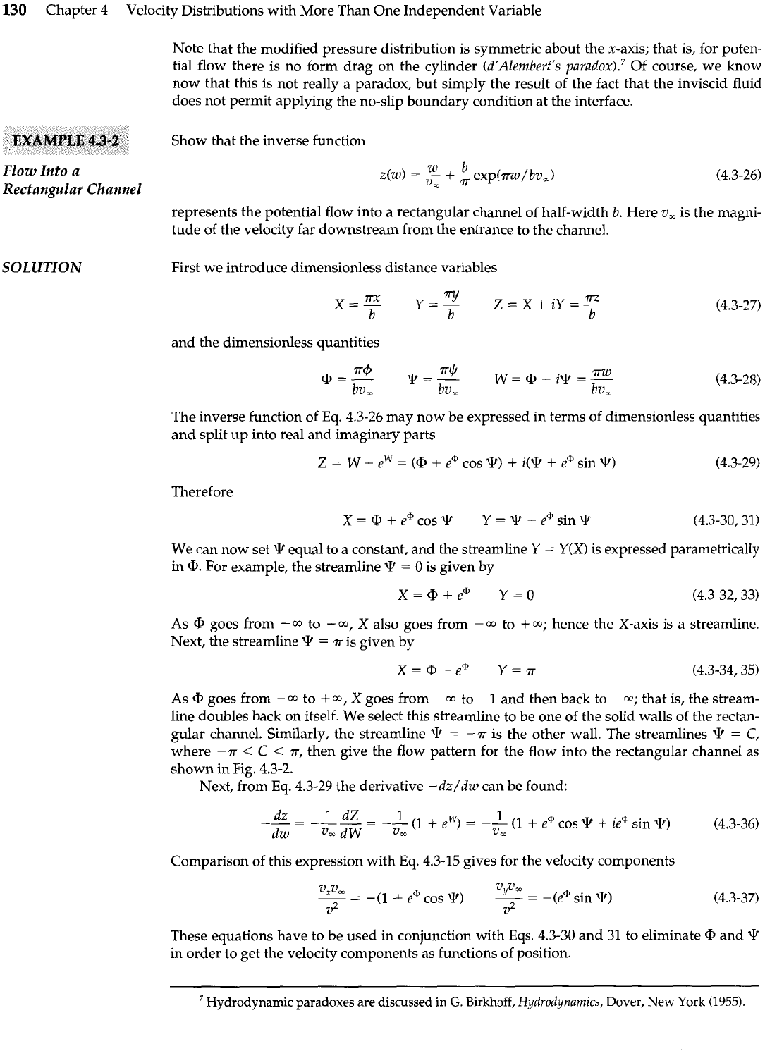
then give the flow pattern for the flow into the rectangular channel

shown in Fig.

4.3-2.

Next, from Eq. 4.3-29 the derivative -dz/dw can be found:

Comparison of this expression with

Eq.

4.3-15 gives for the velocity components

vyvm

-(I

e'cos

- -

(e@ sin

(4.3-37)

These equations have to be used in conjunction with Eqs. 4.3-30 and 31 to eliminate

and

in order to get the velocity components as functions of position.

Hydrodynamic paradoxes

are

discussed

Birkhoff,

Hydrodynamics,

Dover,

New

York

(1955).

94.3

Flow of Inviscid Fluids by Use of the Velocity Potential

131

Flow

Near a Corner8

SOLUTION

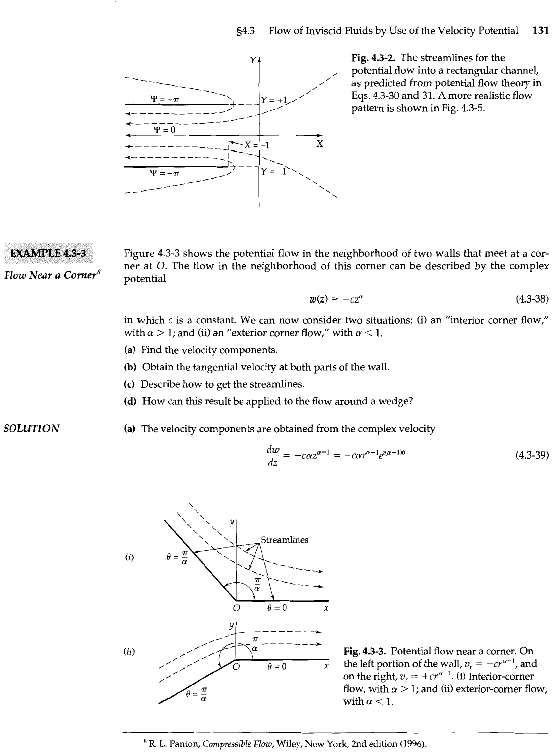
Figure

4.3-3

shows the potential flow in the neighborhood of two walls that meet at a cor-

ner at

The flow in the neighborhood of this corner can be described by the complex

potential

Fig.

4.3-2.

The streamlines for the

in which

is a constant. We can now consider two situations: (i) an "interior corner flow,"

with

and (ii) an "exterior corner flow," with

(a) Find the velocity components.

(b)

Obtain the tangential velocity at both parts of the wall.

(c)

Describe how to get the streamlines.

(d)

How can this result be applied to the flow around a wedge?

---

Y=+T

pG+-Y=

----------

--------

---

Y=O

-I---

(a) The velocity components are obtained from the complex velocity

potential flow into a rectangular channel,

/ /

as predicted from potential flow theory in

Eqs.

4.3-30

and

31.

more realistic flow

+I//

pattern is shown

Fig.

4.3-5.

- - -

(ii)

Fig.

4.3-3.

Potential flow near a corner. On

the left portion of the wall,

-cF1,

and

on the right,

+cua-'. (i) Interior-corner

flow, with

and (ii) exterior-corner flow,

with

- - - -

_/---

----

Panton,

Compressible

Flow,

Wiley,

New

York,

2nd

edition

(1996).

132

Chapter

Velocity Distributions with More Than One Independent Variable

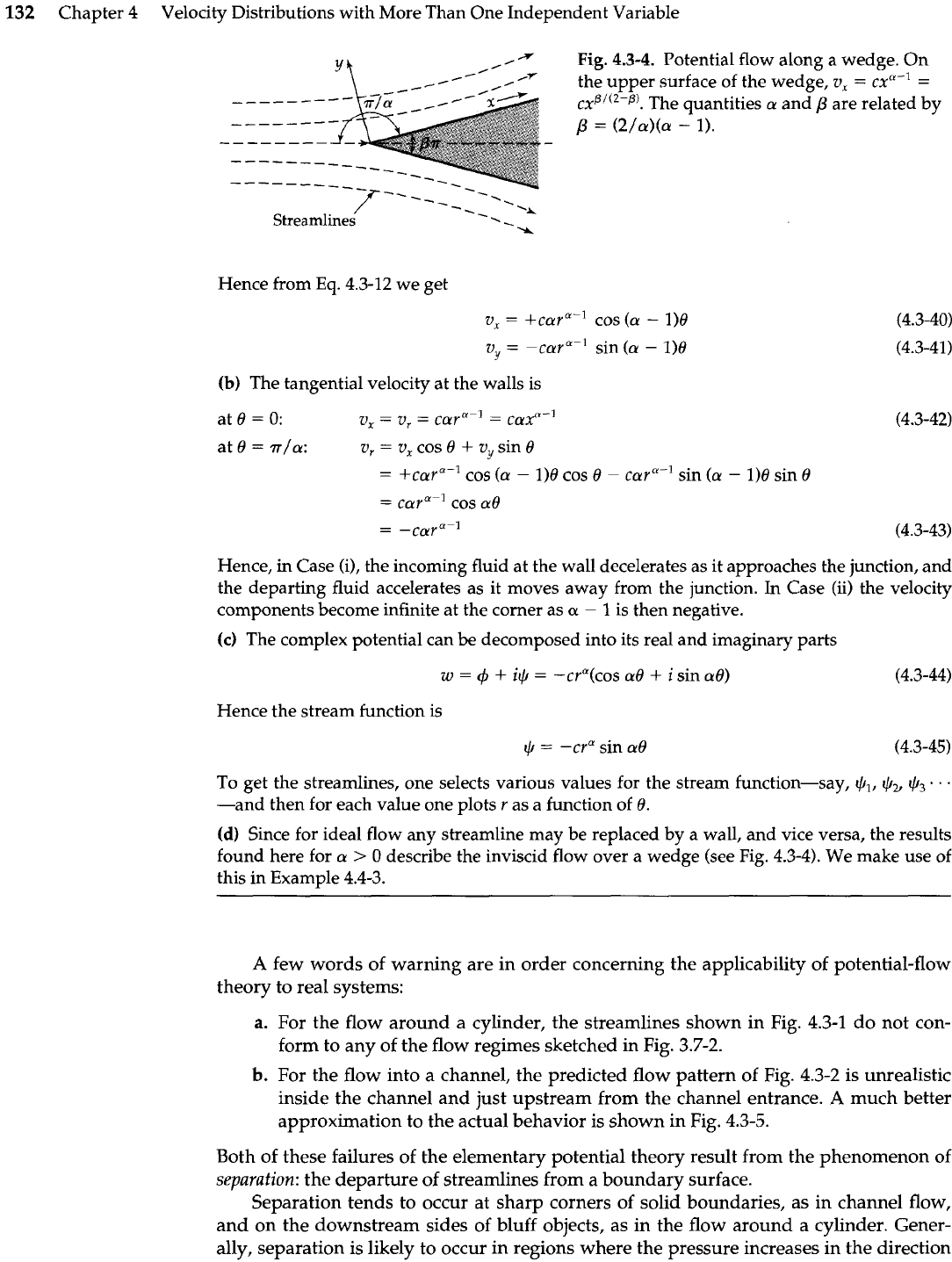
Fig.

4.3-4.

Potential flow along a wedge. On

the upper surface of the wedge,

cxa-'

__-__---

cxP"'-P). The quantities

and

are related by

-------

(2/a)(a

1).

------------

Streamlines

Hence from

Eq.

4.3-12 we get

+cara-' cos

1)6

-cara-' sin

1)6

(b)

The tangential velocity at the walls is

at 0

ZIx

Carn-l

C(yp-l

at 0

r/a:

cos

sin 6

+cara-' cos

1)6 cos 6

cara-' sin

1)6 sin 0

cara-'

COS

- -

-cays-'

(4.3-43)

Hence,

Case (i), the incoming fluid at the wall decelerates as it approaches the junction, and

the departing fluid accelerates as it moves away from the junction. In Case (ii) the velocity

components become infinite at the corner as

is then negative.

(c)

The complex potential can be decomposed into its real and imaginary parts

it,b

-cua(cos a6

sin a61

(4.3-44)

Hence the stream function is

1C,

-cyn sin a0 (4.3-45)

To get the streamlines, one selects various values for the stream function-say,

$,,

t,b,

-and then for each value one plots r as a function of 0.

(d)

Since for ideal flow any streamline may be replaced by a wall, and vice versa, the results

found here for

describe the inviscid flow over a wedge (see Fig. 4.3-4). We make use of

this in Example 4.4-3.

few words of warning are in order concerning the applicability of potential-flow

theory to real systems:

For the flow around a cylinder, the streamlines shown in Fig. 4.3-1 do not con-

form to any of the flow regimes sketched in Fig. 3.7-2.

For the flow into

channel, the predicted flow pattern of Fig. 4.3-2 is unrealistic

inside the channel and just upstream from the channel entrance.

much better

approximation to the actual behavior is shown in Fig.

4.3-5.

Both of these failures of the elementary potential theory result from the phenomenon of

separation:

the departure of streamlines from a boundary surface.

Separation tends to occur at sharp corners of solid boundaries, as in channel flow,

and on the downstream sides of bluff objects, as in the flow around a cylinder. Gener-

ally, separation is likely to occur in regions where the pressure increases in the direction

s4.4

Flow near Solid Surfaces by Boundary-Layer Theory

133

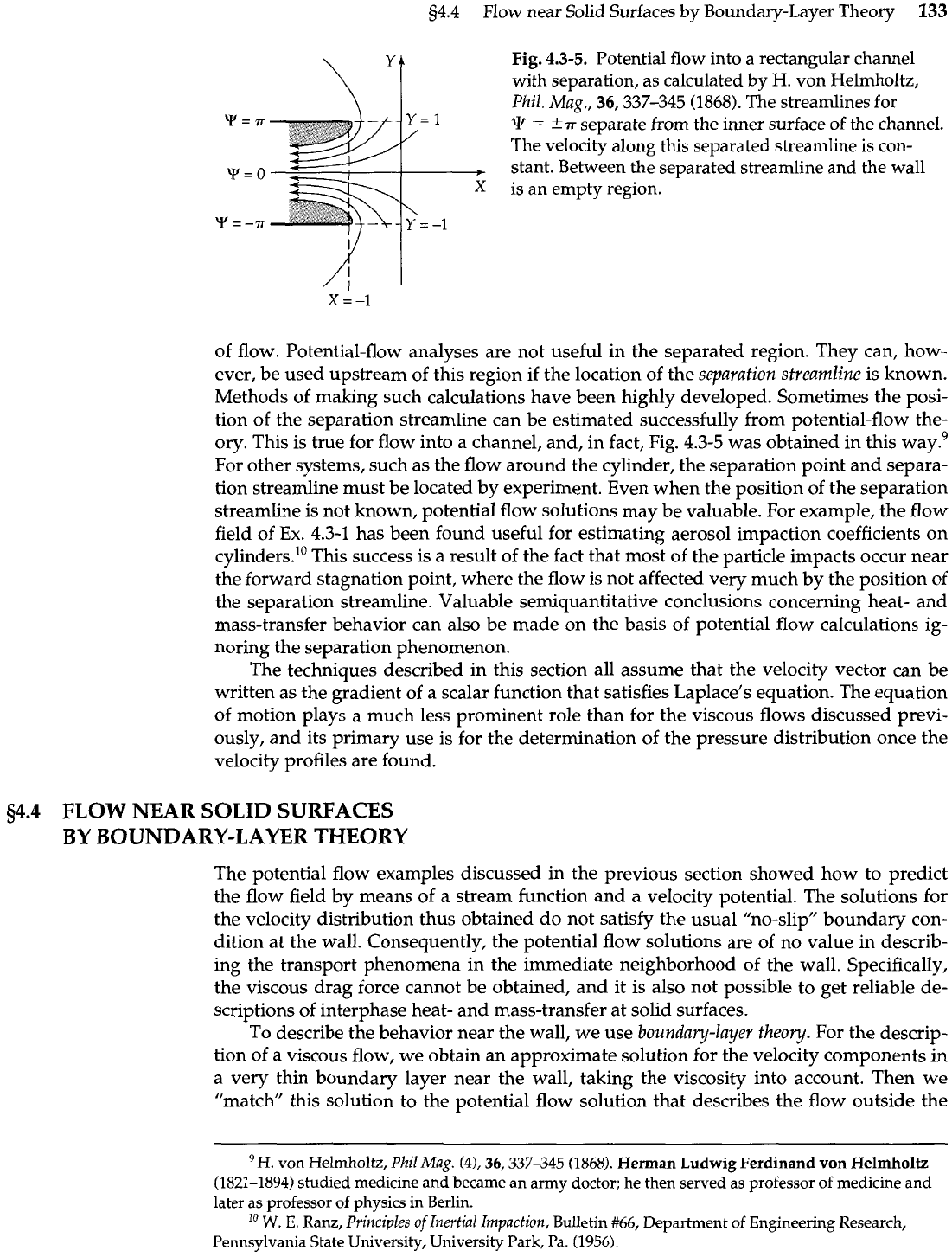
Fig.

4.3-5. Potential flow into a rectangular channel

with separation, as calculated by

von Helmholtz,

Phil.

Mag.,

36,337-345

(1868).

The streamlines for

-+r

separate from the inner surface of the channel.

The velocity along this separated streamline is con-

stant. Between the separated streamline and the wall

X is an empty region.

Y=-7r

of flow. Potential-flow analyses are not useful in the separated region. They can, how-

ever, be used upstream of this region if the location of the separation streamline is known.

Methods of making such calculations have been highly developed. Sometimes the posi-

tion of the separation streamline can be estimated successfully from potential-flow the-

ory. This is true for flow into a channel, and, in fact, Fig.

4.3-5

was obtained in this way.9

For other systems, such as the flow around the cylinder, the separation point and separa-

tion streamline must be located by experiment. Even when the position of the separation

streamline is not known, potential flow solutions may be valuable. For example, the flow

field of

Ex.

4.3-1 has been found useful for estimating aerosol impaction coefficients on

cylinders.1° This success is a result of the fact that most of the particle impacts occur near

the forward stagnation point, where the flow is not affected very much by the position of

the separation streamline. Valuable semiquantitative conclusions concerning heat- and

mass-transfer behavior can also be made on the basis of potential flow calculations ig-

noring the separation phenomenon.

The techniques described in this section all assume that the velocity vector can be

written as the gradient of a scalar function that satisfies Laplace's equation. The equation

of motion plays a much less prominent role than for the viscous flows discussed previ-

ously, and its primary use is for the determination of the pressure distribution once the

velocity profiles are found.

54.4

FLOW NEAR SOLID SURFACES

BOUNDARY-LAYER

THEORY

The potential flow examples discussed in the previous section showed how to predict

the flow field by means of a stream function and a velocity potential. The solutions for

the velocity distribution thus obtained do not satisfy the usual "no-slip" boundary con-

dition at the wall. Consequently, the potential flow solutions

are

of no value in describ-

ing the transport phenomena in the immediate neighborhood of the wall. Specifically,

the viscous drag force cannot be obtained, and it is also not possible to get reliable de-

scriptions of interphase heat- and mass-transfer at solid surfaces.

To describe the behavior near the wall, we use boundary-layer the0

For the descrip-

tion of a viscous flow, we obtain an approximate solution for the velocity components in

a very thin boundary layer near the wall, taking the viscosity into account. Then we

"match this solution to the potential flow solution that describes the flow outside the

von Helmholtz,

Phil

Mag.

(4),

36,337-345

(1868).

Herman Ludwig Ferdinand von Helmholtz

(1821-1894) studied medicine and became an army doctor; he then served as professor of medicine and

later as professor of physics in Berlin.

Ranz,

Principles

Inertial Impaction,

Bulletin

#66,

Department of Engineering Research,

Pennsylvania State University, University Park, Pa. (1956).

134

Chapter

Velocity Distributions with More Than One Independent Variable

boundary layer. The success of the method depends on the thinness of the boundary

layer, a condition that is met at high Reynolds number.

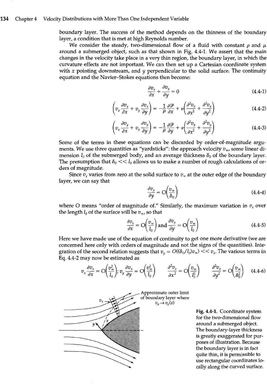
We consider the steady, two-dimensional flow of a fluid with constant

and

around a submerged object, such as that shown in Fig. 4.4-1. We assert that the main

changes in the velocity take place in a very thin region, the boundary layer, in which the

curvature effects are not important. We can then set up a Cartesian coordinate system

with x pointing downstream, and

perpendicular to the solid surface. The continuity

equation and the Navier-Stokes equations then become:

dv,

dvy

-+--=o

Some of the terms in these equations can be discarded by order-of-magnitude argu-

ments. We use three quantities as "yardsticks": the approach velocity v,, some linear di-

mension

of the submerged body, and an average thickness 60 of the boundary layer.

The presumption that So

allows us to make a number of rough calculations of or-

ders of magnitude.

Since

varies from zero at the solid surface to v, at the outer edge of the boundary

layer, we can say that

where

means "order of magnitude of." Similarly, the maximum variation in

over

the length

of the surface will be v,, so that

Here we have made use of the equation of continuity to get one more derivative (we are

concerned here only with orders of magnitude and not the signs of the quantities). Inte-

gration of the second relation suggests that

0((6,/1,)v,)

v,. The various terms in

Eq. 4.4-2 may now be estimated as

v--=O- v-=O--

d2vx

d2v,

(3;

((r)

O(t)

O($) (4.4-6)

dx dx2

dy2

Approximate outer limit

boundary

layer where

VJX)

Fig.

4.4-1.

Coordinate system

for the two-dimensional flow

around a submerged object.

The boundary-layer thickness

is greatly exaggerated for pur-

poses of illustration. Because

the boundary layer is in fact

quite thin, it is permissible to

use rectangular coordinates lo-

cally along the curved surface.

54.4

Flow near Solid Surfaces by Boundary-Layer Theory

135

This suggests that d2vX/dx2

d2vx/dy2,

that the former may be safely neglected. In

the boundary layer it is expected that the terms on the left side of Eq. 4.4-2 should be of

the same order of magnitude as those on the right side, and therefore

The second of these relations shows that the boundary-layer thickness is small compared

to the dimensions of the submerged object in high-Reynolds-number flows.

Similarly it can be shown, with the help of Eq. 4.4-7, that three of the derivatives in

Eq. 4.4-3 are of the same order of magnitude:

Comparison of this result with Eq. 4.4-6 shows that

d9/dy

dP/dx. This means that

the y-component of the equation of motion is not needed and that the modified pressure

can be treated as a function of

alone.

As a result of these order-of-magnitude arguments, we are left with the Prandtl

boundary layer equations:'

(continuity)

(motion)

The modified pressure 9(x) is presumed known from the solution of the corresponding

potential-flow problem or from experimental measurements.

The usual boundary conditions for these equations are the no-slip condition

(v,

O),

the condition of no mass transfer from the wall (vy

0 at

O),

and the

statement that the velocity merges into the external (potential-flow) velocity at the

outer edge of the boundary layer (vx(x,

v,(x)). The function v,(x) is related to 9(x)

according to the potential-flow equation of motion in Eq. 4.3-5. Consequently the term

-(1 /p)(dY /dx) in Eq. 4.4-10 can be replaced by v,(dv,/dx) for steady flow. Thus Eq. 4.4-10

may also be written as

dv, dv, dv, d2v,

vx-+v -=v,-+

V-

ay2

The equation of continuity may be solved for v, by using the boundary condition that

0 at

(i.e., no mass transfer), and then this expression for v, may

substituted

into Eq. 4.4-11 to give

dv, dv, d2v,

vX3- dx

(/,

iildy)%= veZ+

This is a partial differential equation for the single dependent variable vx.

Ludwig

Prandtl(18751953) (pronounced "Prahn-t'l), who taught in Hannover and Gottingen and

later served as the Director of the Kaiser Wilhelm Institute for Fluid Dynamics, was one of the people

who shaped the future of his field at the beginning of the twentieth century; he made contributions to

turbulent flow and heat transfer, but his development of the boundary-layer equations was his crowning

achievement.

Prandtl,

Verhandlungen des III Internationalen Mathematiker-Kongresses

(Heidelberg, 19041,

Leipzig,

pp.

484-491;

Prandtl,

Gesammelte Abhandlungen,

Springer-Verlag, Berlin (1961),

pp.

575-584.

For an introductory discussion of matched asymptotic expressions, see

Acheson,

Elementary Fluid

Mechanics,"

Oxford University Press (1990), pp. 269-271. An exhaustive discussion of the subject may be

found in

Van Dyke,

Perturbation Methods in Fluid Dynamics,

The Parabolic Press, Stanford,

Cal.

(1975).

136

Chapter 4

Velocity Distributions with More Than One Independent Variable

This equation may now be multiplied by

and integrated from

give the

van Ka'rmhn momentum balance2

Here use has been made of the condition that v,(x,

v,(x) as

The quantity on

the left side of

Eq.

4.4-13 is the shear stress exerted by the fluid on the wall:

-~,,l~=~.

The original Prandtl boundary-layer equations, Eqs. 4.4-9 and 10, have thus been

transformed into Eq. 4.4-11,

Eq.

4.4-12, and

Eq.

4.4-13, and any of these may be taken as

the starting point for solving two-dimensional boundary-layer problems. Equation 4.4-

13, with assumed expressions for the velocity profile, is the basis of many "approximate

boundary-layer solutions" (see Example 4.4-1). On the other hand, the analytical or nu-

merical solutions of Eqs. 4.4-11 or 12 are called "exact boundary-layer solutions" (see

Ex-

ample 4.4-2).

The discussion here is for steady, laminar, two-dimensional flows of fluids with con-

stant density and viscosity. Corresponding equations are available for unsteady flow,

turbulent flow, variable fluid properties, and three-dimensional boundary

Although many exact and approximate boundary-layer solutions have been ob-

tained and applications of the theory to streamlined objects have been quite successful,

considerable work remains to be done on flows with adverse pressure gradients (i.e.,

positive

dP/dx)

Eq.

4.4-10, such as the flow on the downstream side of

blunt object.

In such flows the streamlines usually separate from the surface before reaching the rear

of the object (see Fig. 3.7-2). The boundary-layer approach described here is suitable for

such flows only in the region upstream from the separation point.

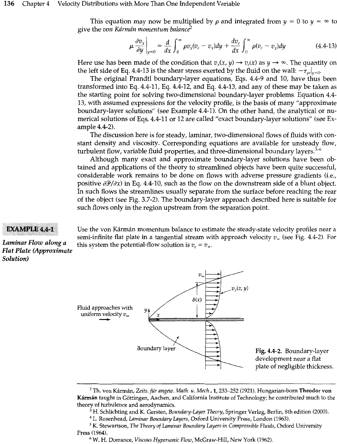
Use the von K5rm6n momentum balance to estimate the steady-state velocity profiles near a

semi-infinite flat plate in a tangential stream with approach velocity

(see Fig. 4.4-2). For

Laminar

this system the potential-flow solution is

a,.

Flat Plate (Approximate

Solution)

Fluid approaches with

uniform velocity

Fig.

4.4-2.

Boundary-layer

development near a flat

plate of negligible thickness.

Th.

von Ksrmin,

Zeits, fur angew. Math. u. Mech.,

1,233-252 (1921). Hungarian-born Theodor von

Kh6n

taught in Gottingen, Aachen, and California Institute of Technology; he contributed much to the

theory

turbulence

and aerodynamics.

Schlichting and

Gersten,

Boundary-Layer Theory,

Springer Verlag, Berlin, 8th edition (2000).

Rosenhead,

Laminar Boundary Layers,

Oxford University Press, London (1963).

Stewartson,

The

Theory of Laminar Bounday Layers in Compressible Fluids,

Oxford University

Press

(1964).

Dorrance,

Viscous Hypersonic Flow,

McGraw-Hill, New York (1962).