Bhattacharjee J.K., Bhattacharyya S. Non-Linear Dynamics Near and Far from Equilibrium

Подождите немного. Документ загружается.

4.2 Self Consistent Mode Coupling 91

will be generated, but one particular set of diagrams will be simply an iteration of

the lower order one, i.e. graphs of the structure shown in Fig. 4.4

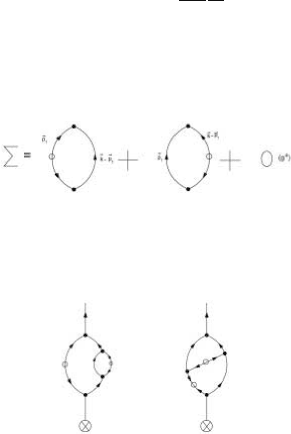
Figure 4.4. A two loop disconnected response function

With these structures repeating at every order

G(k, ω) = G

(0)

(k, ω) −g

(0)

(k, ω)

(k, ω)G

(0)

(k, ω)

+ g

(0)

(k, ω)

(k, ω)G

(0)

(k, ω)

(k, ω)G

(0)

(k, ω) +.........

= G

(0)

(k, ω) −g

(k, ω)G(k, ω)

leading to

G(k, ω) =

(0)

(k, ω)

1 +g

(k, ω)G

(0)

(k, ω)

−1

(k, ω) =G

(0)

−1

(k, ω) + g

(k, ω) (4.2.13)

which is just the Dyson’s equation for the problem. It is convenient to write

Eq.(4.2.13) as

−1

(k, ω) =−

iω



(k, ω)

= (

)

−1

[−iω +

) +(k, ω)] (4.2.14)

where

(k, m, ω) = g

)



(2π)

−p

)

)(p

)

−iω +

) +

)

+O(g

)

(4.2.15)

92 4 Mode Coupling Theories

It is convenient to write this answer as an integral over the correlation function as

(k, m, ω) = g

)



+ω

=ω

p

+p



(2π)

dω

2π

−p

)

× C

(0)

( p

,ω

(0)

( p

,ω

) +O(g

) (4.2.16)

It should be noted, however, that the possibility of writing the self-energy (k, ω)

in the form of Eq.(4.2.16) as an integral over correlation function is a consequence

of the FDT. The general structure is that shown in Fig. 4.3. The self-energy is

extracted from the graphs by removing the external lines and in Fig. 4.4, we show

the generally true form of the self-energy at this order

Figure 4.5. The one loop self energy

It should be noted that in writing Eq.(4.2.13) one has included graphs of the

form chosen in Fig. 4.4 (technically called reducible - because a cut across the

connecting propagator would divide the graph into two) but has left out graphs of

the form shown in Fig. 4.6.

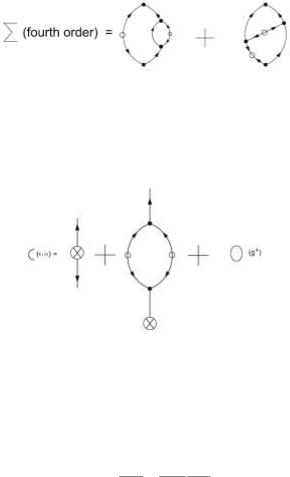
Figure 4.6. The two loop response function

Graphs for G such as shownin Fig. 4.6 would contributeat O(g

) to (k, m, ω)

and the corresponding contributions would be as shown in Fig. 4.7

4.2 Self Consistent Mode Coupling 93

Figure 4.7. The two loop contributions to the self energy

We have not shown all the possibilities at the fourth order.

Because of the FDT, we do not need to set up separately the perturbation theory

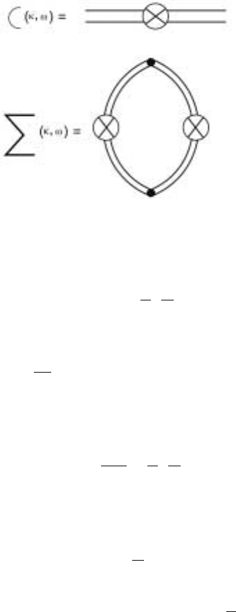
for the correlation function. When there is no FDT, this needs to be done and the

discussion that we have had so far, when carried out for C(k,ω) to the expansion

shown in Fig. 4.8

Figure 4.8. The one loop correlation function

We now turn to the physical signiﬁcance of the self-energy (k, ω) This is best

done by referring to Eq.(4.2.14). The self-energy, as is evident from that equation

is an addition to 

) the relaxation rate in the linearized theory. Thus

(k, ω) is the contribution to the relaxation rate coming from the nonlinear terms.

We now turn to Eq.(4.2.15) to estimate how big the contribution is. We work at

m =0 (critical point), ω =0 (long time) and consider the long wavelength limit

(k →0). The self-energy becomes

(k) g

2D



(2π)

1+D

dp (4.2.17)

In the above the limit k →0, makes

p

94 4 Mode Coupling Theories

and

−p



k. p.

also

cos

θ=

The integral converges at the lower limit for D>6 but for D<6, has to be cut off

at p k to prevent the divergence. So (k) has a long wavelength divergence for

D<6 and in this limit the non-linear contribution to the relaxation rate completely

dominates the linear contribution 

. When the nonlinear terms dominate, we

have (keeping the normalization G

−1

(k, 0) =χ

−1

)

−1

(k, ω) =[−iω +(k, ω)]

−1

(k, 0)

(4.2.18)

For the ferromagnet this happens at D<6. For D>6, the nonlinear terms do

not affect the momentum dependence of the relaxation rate as obtained from the

linearized model and the nonlinear terms are irrelevant. Thus D =6 is the upper

critical dimension. This is exactly the same as we found from the RG treatment in

Chapter 3.

We are now ready to convert the perturbative result of Eq.(4.2.16) into a non

perturbative one. We assume that the perturbative  on the L.H.S of Eq.(4.2.16)

will become the full , if we replace the bare correlation functions on the R.H.S

by the full correlation function C(k,ω). Because of the FDT, the full C(k,ω) is

related to the full G(k, ω) and hence to the (k, ω). Thus we have,

(k, ω) = (k



(2π)

dω



2π

C( p, ω



)



k −p, ω −ω



)[p

−(



k −p)

]

C(k,ω) =

Im G(k, ω)

and G

−1

(k, ω) =[−iω +(k, m, ω)]

−1

(k, m)

(k, m)

(4.2.19)

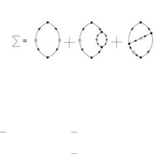
The above set of equations determine the self energy in a self consistent manner.

The diagrammatic representation of the above equation is shown if Fig. 4.9. This

technique of ﬁnding (k, ω) is called the self consistent mode coupling approxi-

mation.

(When FDT is not valid, the self consistent mode coupling would involve the

lines in the self energy part of Fig. 4.3 represent the full Green’s function and the

full correlation function.)

4.2 Self Consistent Mode Coupling 95

Figure 4.9. The one loop dressed correlation function

We now ask whether Eq.(4.2.19) has a scaling solution. This involves writing

(k, ω)=k





(4.2.20)

with the constraint



C(k,ω)

dω

2π

=χ(k)=k

−2

for m =0

the dimension of C(k,ω) is k

−2−z

(the frequency corresponds to k

) i.e. the scaling

form of C(k,ω)

C(k,ω) =

2+z





(4.2.21)

The power count of the integral on the R.H.S in Eq.(4.2.20) gives k

2+D−z

. The

L.H.S is k

and matching immediately leads to

z =1 +

(4.2.22)

for D<6, exactly as in the RG treatment of Chapter 3.

We now ask how much can one infer about the function f(

) in Eq.(4.2.20). At

the critical point and at ω =0, the function is a constant , i.e. (k,0) =k

and

one needs to ﬁnd the value of . In general the determination of the function f has

to be done numerically from Eq.(4.2.19). However, we show here that for D 6,

there is an analytic solution. For D =6, referring to Eq.(4.2.17) the integral on the

R.H.S will be dominated by the high momenta and the self energies on the R.H.S

of the integral in Eq.(4.2.19) are effectively at zero frequency and we can write

96 4 Mode Coupling Theories

C(k,ω) =

χ(k)

2(k)

[

−iω +(k)

iω +(k)

] (4.2.23)

This allows the frequency integration in Eq.(4.2.19) to be done and leads to

(k, ω) = g

−1

(k)



(2π)

−(



k −p)

]

(



k −p)

−iω +( p) +(



k −p)

(4.2.24)

Since the self consistency of the above approach is for high values of the internal

momentum p, we can carry out the high momentum approximation in the integrand

of the above equation. For ω =0, and remembering that D 6,

k

= g

(2π)

2



∞

D−1

= g

(2π)

2



∞

4−



(2π)



(4.2.25)

where  =6 −D. Thus



(2π)



(4.2.26)

for  1, which is exactly identical to Eq.(4.2.24) obtained from the RG technique.

Thus, if the self consistent mode coupling equations are solved by iterating around

the upper critical dimension, one obtains a perturbation series which matches ex-

actly the perturbative RG result.

Before ending this section, we note that making the Ansatz of Eq.(4.2.23) for

the correlations functions on the R.H.S. of Eq.(4.2.19) is a ﬁrst step in an iterative

process of situation and is in general a very effective technique for obtaining a

solution. With this approximation for C(k,ω), the self-energy (k, ω) is given in

general by,

(k, m, ω) = g

−1

(k, m)



(2π)

−p

)

−iω +(p

,m)+(p

,m)

(4.2.27)

As we have already seen, for m =0 and ω =0,

(k, ω)=k

4.2 Self Consistent Mode Coupling 97

Now for m k, we need to ﬁnd out (k, m). Inspection of Eq.(4.2.27), shows that

the integral is proportional to k

and we anticipate

(k, m) ∼k

for m k.

Self consistency of Eq.(4.2.27) requires

(k, m) = g

(2π)



D−1

)

2(p,m)

= g

(2π)

D−1

)

∝ m

D−2−y

, (4.2.28)

leading to

y =

−1 (4.2.29)

We now investigate another limit, namely the case of very high frequency, i.e.

ω  k

or ω 

k

−1

In this limit, k and m both tend to zero and appropriate approximations in

Eq.(4.2.27), lead to

(k, ω) = g

(2π)



D−1

[−iω +2(p)]

= g

(2π)



D−3

−i

= g



−iω



3−D/2

1+D/2

(2π)



7D −4

2(2 +D)

12 −5D

2(2 +D)



(4.2.30)

With the above limiting forms for (k, m, ω), we have the following results:

(k, m, ω) =k

)L(k, m, ω) (4.2.31)

where

L(k,m,ω) ∝ k

−/2

for m =ω =0

∝ m

−/2

for k =ω =0

∝ (

−iω

)

−



2+D

for k =m =0 (4.2.32)

where  =6 −D

98 4 Mode Coupling Theories

4.3 Spherical Limit

In this section, we discuss an approximation that was invented forty years ago for

problems in non-linear dynamics buthas attracted attention only recently. This is the

spherical limit. It has been a popular approximation in static critical phenomena

for more than two decades, but its place in dynamics was not appreciated until

recently. There are some contemporary ways of introducing this technique, but we

will use the very general framework that Kraichnan used in his pioneering work,

and cast it in a language appropriate to the discussion of the Heisenberg model

with which we have demonstrated both the RG and self consistent mode coupling

techniques. Our equation of motion is, in momentum space

(k) =−k

)φ



p

+p





ij l

−p

)φ

( p

)φ

( p

) +N

N

(k, ω)N



,ω



)=2k

(



k +





)δ(ω +ω



) (4.3.1)

To set up a spherical limit, one needs to introduce a M-component generalization

of the above dynamical system. Kraichnan’s method is to introduce M-copies of

the system with the magnetization vector for the m

copy being denoted by



[m]

A collective coordinate



is now deﬁned as



√



m=1

2παm/M



[m]

(4.3.2)

This index α runs from −s to s in steps of unity with 2 s +1 =M. One now needs

to introduce an equation of motion



, which will reduce to Eq.(4.3.1) if M =1.

The required equation of motion is

(



k) =−k

)φ

(α)

(k) +

√



p

+p





ij l



α,β,α−β

−p

)φ

(β)

( p

)φ

(α−β)

( p

) +N

N

(α)

(k, ω)N

(β)



,ω



)=2k

(



k +





)δ(ω +ω



)δ

αβ

(4.3.3)

The coupling λ

α,β,α−β

are endowed with the following properties

• i) λ

α,β,α−β

=λ

α,α−β,β

• ii)λ

α,β,α−β

=1 if anyone of the subscripts is zero

• iii)λ

α,β,α−β

=λ

∗

−α,−β,−(α−β)

• iv)λ

∗

α,β,α−β

=λ

α−β,−β,α

=λ

β,α,−(α−β)

4.3 Spherical Limit 99

The second condition ensures that Eq.(4.3.4) reduces to Eq(4.3.1) for M =1. Thus

Eqns.(4.3.3)are a proper generalization of Eqns.(4.3.1). The ﬁrst constraint written

down above expresses a natural symmetry of the system, namely in the coupling

of modes on the R.H.S of Eq.(4.3.3) it does not matter whether the mode with

momentum p

belongs to the β

or the (α −β)

replica of the system. The third

constraint ensures that in the course of evolution, the ﬁeld



remains real. This is

done by demanding that the equation of motion for



, corresponding to Eq.(4.3.3),

the non-linear term remains real. The fourth constraint above is obtained from the

fact there must exist an equilibrium probability distribution at all times for doing

averages. For the replicated system, this distribution corresponds to the action

(“free energy”)

F =



(k)φ

(−k)(k

)

and the equation of motion must remain

=0.

For this to hold under Eq.(4.3.3), we must have the fourth constraint.

It should be noted that the procedure carried out so far is absolutely general and

can be carried through any dynamical system.The idea is to introduce M replicas

and coupling between the replicas in the non-linear term in a manner such that the

correct equation of motion is obtained for M =1. We now introduce the vital step

that will allow the model to be exactly solvable for M →∞and it should be noted

that this step too is very general and can be carried out for any system. This step

constitutes writing

α,β,α−β

iθ

α,β,α−β

(4.3.4)

where the phase factors θ

α,β,α−β

take a value randomly between 0 and 2π for every

assigned value of α and β.

The task of the theory is to calculate the self-energy G(k, ω), which we learnt

in the previous section can be written as

−1

(k, ω) =−iω +k

) +(k, ω)

where (k, ω) has an expansion in powers of g. The complete terms of O(g

) are

shown in Fig. 4.5 and the typical fourth order term (i.e. O(g

)) terms are shown in

Fig. 4.7. In Fig. 4.9, we show the same diagrams with two contributions of Fig. 4.5

combined into one and some similar combinations carried out in Fig. 4.7.

Imagine constructing 

αα

where α is a ﬁxed replica index. We ﬁrst consider the

O(g

) calculation corresponding to graph (a) in Fig. 4.10. The coupling constant

brings in g

/M. Now the mode α connects to modes β and α −β. Since the noise

correlation involves the same replica (see Eq.(4.3.3)), if the λ factor at one vertex

100 4 Mode Coupling Theories

Figure 4.10. The two lowest orders for the self energy

is λ

α,β,α−β

, then at the other it has to be λ

β,β−α,α

. Thus, the replica part of the

contribution to  is



β=1

α, β, α−β

β, β−α, α



β=1

α, β, α−β



β=1

∗

α, β, α−β



β=1

|λ

α, β, α−β

(Using (iv) and (i))

= 1

where we have used Eq.(4.3.4) in arriving at the last line. This the contributions of

Fig. 4.10a to (k, ω) is O(1).

Turning to the contribution of graph(b) of Fig. 4.10, we note that these are two

independent free replica indices left to sum over after the preliminary algebra.

These correspond to the line on the left to the graph( b) and one of the lines in the

sub graph on the right hand line Fig 4.10b. These two sums provide a factor M

while the four



vertices each come with a factor of M

−1/2

and thus produce

−2

. Consequently, this contribution is O(1).

Now, consider the contribution from Fig. 4.10c. The four vertices produces

factors which can be written as the string



β,γ

α, β, α−β

β, γ, β−γ

γ,β−α, γ +α−β

β−γ,β−γ −α, α

Note that every time, we choose a value of β, the γ -value has to be ﬁxed at

γ =2β −α, so that the λ factors can combine to produce |λ|

=1. If it did not

do this, then the sum over indices would produce zero due to the random phase

averaging introduced following Eq.(4.3.4). Thus β and γ are not independent.

Hence the double sum in the string produces a factor of M only and the contribution