Bennett A.F. Inverse Modeling of the Ocean and Atmosphere
Подождите немного. Документ загружается.

5.2 Ocean tides 127
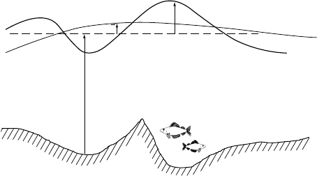
H
h
h
Figure 5.2.2 Shallow-
water theory.
Note 3. Many more effects can be included, yielding real gains in forecast accuracy.
These include
(i) load tide: as sea level rises and falls, the ocean floor subsides and rebounds
elastically;
(ii) earth tides: the tgf directly drives motions in the elastic earth;
(iii) self tide: as sea levels rises, the local accumulation of mass deflects the local
vertical;
(iv) geoid corrections: the earth tides change the shape of the earth and hence that
of the earth’s geopotentials or “horizontals”;
(v) atmospheric tides: the tgf and solar heating drive motions in the atmosphere
which perturb sea-level pressure.
The LTEs require boundary conditions, such as
u ·
ˆ
n = 0 (5.2.4)
at coasts, or
h = h
B
(5.2.5)
at an open boundary. These are unsatisfactory: is the boundary at the shore line or
the shelf break? Can h
B
be measured economically? How shall we avoid spurious
oscillations in an open region, when the LTEs are subjected to (5.2.5)?
5.2.4
Tidal data
Tides are the best measured of all ocean phenomena. The data include:
(i) century-long high-quality time series of sea level at about one hundred coastal
stations, measured with floats in “stilling wells” and strip-chart recorders;
(ii) year-long high-quality time series of bottom pressure in about twenty deep
ocean locations, measured with the piezoelectric effect and digital recorders;
(iii) year-long good-quality time series of ocean current at selected depths at about a
thousand deep locations;
128 5. The ocean and the atmosphere
d uXst dX s
s
s
=
()
⋅+∈
∫
1
2
((), )
X(s
1
)
X(s)
X(s
2
)
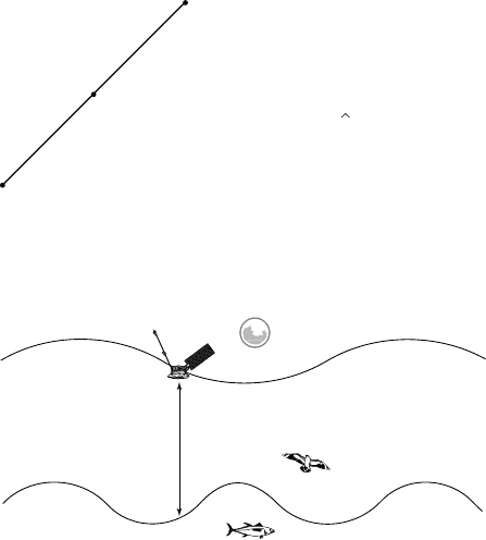
Figure 5.2.3 Reciprocal-
shooting tomography.
orbit
sea level
GHz radar travel-time
Figure 5.2.4 Satellite radar
altimetry.
(iv) year-long good-quality time series of reciprocal-shooting acoustic tomography
at about a dozen deep ocean locations: see Fig. 5.2.3.
(v) satellite altimetry: see Fig. 5.2.4.
Altimetric missions include GEOSAT, ERS-1 and TOPEX/POSEIDON. The last
(T/P) has a ten-day repeat-track orbit from 70
◦
Sto70
◦
N approx.: see Fig. 5.2.5.
Again, TOPEX/POSEIDON has been flying and operating successfully since August
1992.
Temporal variability in the orbit of T/P is known with remarkable precision:
±2 cm. However, the shape of the gravitational equipotential (the “geoid”) is not known
so accurately. This bias can be eliminated from the data by considering “cross-over”
differences: see Fig. 5.2.6. The datum becomes
d = h(X, T
D
) − h(X, T
A
) + .
Note that T
A
and T
D
need not be the times of consecutive passes over X. The values
of |T
A
− T
D
|for consecutive passes can be as large as five days, thus semi-diurnal tides
are severely aliased. In fact, the aliased tides resemble Rossby waves with periods of
about 60 days. We shall use the dynamics of the LTE to identify and hence reject the
aliased tides, which have great spatial coherence.
Figure 5.2.5 TOPEX orbits.
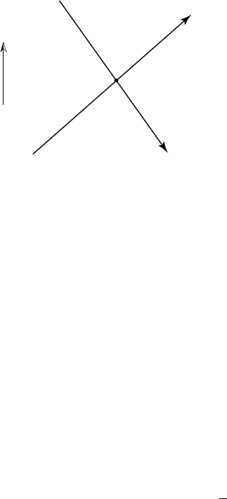
130 5. The ocean and the atmosphere
N
X
Ascending (A)
Descending (D)
Figure 5.2.6 Orbit
cross-overs.
5.2.5 The state vector, the cross-over measurement
functional and the penalty functional
Let us work with tidal volume transports U
k
(x) ≡ H (x)u
k
(x) and elevations h
k
(x)at
frequency ω
k
, for 1 ≤ k ≤ K . Then the state vector field is
U = U(x) =
U
1
h
1
U
2
h
2
.
.
.
.
.
.
U
K
h
K
∈ CCCC
3K
. (5.2.6)
Recall that U
k
and h
k
are complex-valued. The dynamics become
iω
k
U
k
+ f
ˆ
k × U
k
+ gH∇(h
k
− h
k
) +rU
k
/H = ρ
k
, (5.2.7)
iω
k
h
k
+ ∇ · U
k
= σ
k
, (5.2.8)
where ρ
k
and σ
k
are dynamical misfits or residuals. Note that the bathymetry H only
appears in the momentum equation, so the continuity equation should be very accurate.
The boundary conditions are
U
k
·
ˆ
n
∼
=
0 at coasts, h
k
∼
=
h
B
k
at open boundaries. (5.2.9)
We refrain from introducing symbols for the boundary residuals; instead we shall
express (5.2.7)–(5.2.9) compactly as
SU = F + τ , (5.2.10)
where S comprises the linear dynamical operators and linear boundary operators, F
includes the tgf and boundary forcing, while τ includes the dynamical and boundary
residuals.

5.2 Ocean tides 131
The cross-over data involve the linear measurement functional
L
m
[U] = h
X
m
, T
(2)
m
− h
X
m
, T
(1)
m
, (5.2.11)
where X
m
is a cross-over location, while T
(1)
m
and T
(2)
m
are the times of distinct passes.
Note that L
m
selects only the elevation h, and evaluates it at certain times. In terms of
complex harmonic amplitudes, the functional becomes
L
m
[U] = e
K
k=1
h
k
(X
m
)
e
iω
k
T
(2)
m
− e
iω
k
T
(1)
m
, (5.2.12)
for 1 ≤ m ≤ M. In compact form, the data are
d = L[U] + . (5.2.13)
Note that the field U has values in CCCC
3K
, while d belongs to RRRR
M
.
Exercise 5.2.2
Devise the measurement functionals for data types (i)–(iv) in §5.2.3. Explain why
representers for altimetric cross-over data can be constructed using representers for
tide gauge data.
Finally, the penalty functional for inversion of the LTE and T/P data is (Egbert
et al., 1994; Egbert and Bennett, 1996)
J [U] = τ
∗
◦ W
τ
◦ τ +
∗
w, (5.2.14)
where
∗
denotes the transposed complex conjugate vector. Note that we should choose
W
τ
= C
−1
τ
, where C
τ
is the covariance of residuals at different places and at different
frequencies, and we should choose w = C
−1
where C
is the covariance of measure-
ment errors.
5.2.6
Choosing weights: scale analysis of dynamical errors
Before proceeding with the mathematical task of minimizing the penalty functional J ,
let us take a first look at the choice of weights in J . As these will be the inverses of
error covariances, consider first some scale estimates of dynamical errors.
(i) The dynamics are linearized. Also, we have analyzed the fields harmonically,
thus
∂h
∂t
= i ωh at frequency ω. Let us assume that
∂h
∂x
∼ κδh, where κ is some
wavenumber and δh is the rough magnitude of h. The balance between local
accelerations and pressure gradients (5.2.7) may be expressed as
ωδu ∼ gκδh. (5.2.15)

132 5. The ocean and the atmosphere
The balance between the local rate of change of sea level and the convergence
of volume flux in (5.2.8) is
ωδh ∼ κ H δu. (5.2.16)
Hence
ω
2
∼ gHκ
2
,κ∼
ω
c
, (5.2.17)
where c = (gH)
1
2
, and
δu ∼
ωδh
κ H
∼
+
g
H
,
1
2
δh = c
δh
H
. (5.2.18)
Now compare the local acceleration and momentum advection in (5.2.7):
ωδu : κ(δu)
2
. (5.2.19)
These are in the ratio
1:
κδu
ω
, or 1 :
δu
c
, or 1 :
δh
H
. (5.2.20)
The linearization error in the continuity equation (5.2.8) is also (δh/H ). In deep
water H ∼ 5000 m and δh ∼ 0.2 m, so linearization is highly accurate. Note
that c = (gH)
1
2
∼ 200 m s
−1
,soδu ∼ 0.008 m s
−1
.
(ii) The pressure gradients in (5.2.7) are derived from the hydrostatic balance (not
shown). Using the three-dimensional incompressibility condition (not shown),
we may deduce that the scale of the vertical velocity is δw ∼ κ H δu, hence the
comparison of local vertical accelerations to the gravitational acceleration is
ωδw : g, or ωκ H δu : g, (5.2.21)
or
cκ
2
Hδu : g, or κ
2
H
2
(δu/c):1. (5.2.22)
So the hydrostatic balance is extremely accurate for small-amplitude
(δh H ), long waves (κ H 1) in deep water. The dynamics are “shallow” in
the sense that κ H 1.
(iii) A crude estimate of numerical accuracy is made by comparing the horizontal
grid spacing x to the length scale κ
−1
= cω
−1
. For solar semidiurnal tides,
ω = 2π
1
2
d
−1
= (2π/43 200) s
−1
∼
=
1.4 × 10
−4
s
−1
,
so κ
−1
∼ 200 m s
−1
/(1.4 × 10
−4
s
−1
)
∼
=
1.4 × 10
6
m = 1400 km. Thus, if
x = 0.5
◦
∼
=
50 km, and the numerics are second-order accurate, then

5.2 Ocean tides 133
truncation errors are entirely negligible. Tidal diffraction at peninsulae reduces
the length scale significantly. It is also common practice to reduce grid spacing
in shallow water according to the rule x ∝ H
1
2
.
Exercise 5.2.3
Justify the shallow-water grid rule given above.
(iv) The mean depth H (x) is commonly taken from the US Navy’s ETOP95
bathymetry, which is available at NCAR. These data are very doubtful at high
latitudes. In the deep North Pacific we can only guess that the error is about
100 m in 5000 m, or 2%. There are known to be far greater errors in, for
example, the Weddell Sea.
(v) We have adopted the crude drag law: iωu ···=···−r u/H, where
r = 0.03 m s
−1
. It is common practice to replace r/H with r/ max[H, 200 m],
in order to avoid excessive drag over the continental shelves. These drag
formulae are usually tuned so that the tidal solutions are in reasonable
agreement with data. Nevertheless, such drag laws are crude parameterizations,
so it is prudent to assume that they are 100% in error. However, the drag is a
very small part of the momentum balance in deep water.
(vi) The rigid boundary condition is simply
Hu ·
ˆ
n = 0, (5.2.23)
where
ˆ
n is normal to the boundary. The question arises: where is the boundary?
In a numerical model the precision of location is no smaller than x,sothe
error in (5.2.23) is of the order of
x
∂
∂n
(H u ·
ˆ
n) ∼ xκ H δu ·
ˆ
n. (5.2.24)
The relative error in (5.2.23) is therefore ∼xκ. If we assume that
κ ∼ ω(gH)
−
1
2
, H ∼ 100 m, g ∼ 10 m s
−2
and ω = S
2
1.4 × 10
−4
s
−1
, then
κ
∼
=
0.5 × 10
−5
m
−1
.Soifx = 0.5
◦
∼
=
50 km, then
xκ
∼
=
0.25. (5.2.25)
The relative error in (5.2.23) is 25%! The depth would have to increase to
10 km in order for xκ to be as small as 2.5% (given x = 0.5
◦
). So rigid
boundary conditions are significant sources of error in numerical tidal models.
The solution in mid-ocean may not be sensitive to this error source, as the basin
resonances are very broad. That is, the coastal irregularity itself ensures a fine
spectrum of seiche modes. Finally, the high-resolution Finite Element Model
(FEM) for global tides developed at the Institute for Mechanics in Grenoble,
France is the best forward model yet developed (Le Provost et al., 1994).

134 5. The ocean and the atmosphere
In summary, linearization and truncation errors in the continuity equation are negli-
gible. Bathymetric errors and drag errors in the momentum-transport equations should
be admitted, while rigid boundary conditions are significantly in error.
5.2.7
The formalities of minimization
Let us set aside our preliminary discussion of model errors, and make some notes on
the formalities of minimization. The penalty functional (5.2.14) is
J [U] = τ
∗
◦ C
−1
τ
◦ τ +
∗
C
−1
(5.2.26)
≡ (SU − F)
∗
◦ C
−1
τ
◦ (SU − F) + (d − L[U])
∗
C
−1
(d − L[U]). (5.2.27)
Setting the first variation of J to zero yields
0 =
1
2
δ
ˆ
J = (SδU)
∗
◦ C
−1
τ
◦ (S
ˆ
U − F) − L[δU]
∗
C
−1
(d − L[
ˆ
U]). (5.2.28)
The vanishing of the coefficient of δU
∗
yields
S
†
Λ = L[δ]
∗
C
−1
(d − L[
ˆ
U]), (5.2.29)
where
S
ˆ
U = F + C
τ
◦ Λ. (5.2.30)
Note that S and the adjoint operator S
†
include the dynamics and the boundary
conditions.
Exercise 5.2.4
Derive (5.2.29), (5.2.30) in detail.
Let us now examine L for TOPEX/POSEIDON cross-over data (T/P XO data):
L
m
[U] = h
X
i
, T
(2)
j
− h
X
i
, T
(1)
j
, (5.2.31)
where 1 ≤ m = m(i, j) ≤ M. The X
i
for 1 ≤ i ≤ I are the XO locations; the T
(1,2)
j
for 1 ≤ j ≤ J are the XO times. In terms of tidal constituents we have, from (5.2.12):
L
m
[U] = e
K
k=1
h
k
(X
i
)
e
iω
k
T
(2)
j
− e
iω
k
T
(1)
j
. (5.2.32)
So it suffices to calculate representers for h
k
(X
i
) for 1 ≤ i ≤ I and 1 ≤ k ≤ K . Then
we can synthesize the representers for the (X
i
, T
(1,2)
j
) XO difference. This is very
useful. There are only 1 × 10
4
XO points but by 9/99 there had been approximately
258 ten-day repeat-track orbit cycles, or about 1.8 × 10
6
XO data. According to the
above harmonic analysis, we need only compute K × 10
4
representers (K is usually 4
or 8). How else might we reduce the computations? Inspection of reasonably accurate
solutions of forward tidal models indicates that the XO coverage is unnecessarily dense,
5.2 Ocean tides 135
for observing tides. In the open ocean, adequate coverage is obtained with every third
XO in each direction. Thus we may reduce the number of representers by nearly a factor
of ten. Finally, a cheap preliminary calculation of all the remaining representers, using
a coarse numerical grid, permits an array mode analysis (see §2.5). The analysis shows
that a further reduction by a factor of about four is appropriate. In conclusion, about
4000 real representers are needed. They may be fitted to the 1.8 × 10
6
data values,
however.
5.2.8
Constituent dependencies
It might be inferred from the preceding discussion that the representers at different
tidal frequencies may be calculated independently. In general, this is not the case. The
representer adjoint variables obey
S
†
k
α
k
= δ(x − ξ)
ˆ
e
3
(5.2.33)
for 1 ≤ k ≤ K , where
ˆ
e
3
= (0, 0, 1, 0)
T
, and so may be calculated separately. However
the representers obey
S
k
r
k
=
K
l=1
C
τ
kl
◦ α
l
(5.2.34)
for 1 ≤ k ≤ K , and in general the LTE error covariance is not diagonal with respect to k
and l. Nevertheless, we may reasonably assume that errors for semidiurnal constituents
are independent of those for diurnal constituents. The tidal inverse problem involves
immense detail, because so much is known about the structure of the tide-generating
force.
5.2.9
Global tidal estimates
Estimating global ocean tides using hydrodynamic models and satellite altimetry is
formulated as an inverse problem in Egbert et al. (1994). The altimetric data are
being inverted in order to find errors in the drag law and bathymetry, especially in
the deep ocean. Linear dynamics and linear measurement functionals suffice. The time
dependence involves few degrees of freedom and those are highly regular, pure har-
monic in fact. The number of cross-over data and hence the number of representers is
very large (and still growing, after eight years), yet their number can be reduced by
obvious and reasonable subsampling strategies (for example, every third cross-over in
each direction), and by a priori array assessment based on economical computation of
representers on a coarser numerical grid. The eventual set of decimated and rotated
representers may still be fitted closely to the entire data set, however.
Best of all, the challenge of a real, large and important problem led (Egbert, personal
communication) to the indirect representer method, outlined in §3.1.3 and applied to real
136 5. The ocean and the atmosphere
data in Egbert et al. (1994; hereafter referenced as EBF). This tidal solution and others
have been extensively reviewed (Andersen et al., 1995; Le Provost, 2001; Le Provost
et al., 1995; Shum et al., 1997). The solutions were tested with independent tide gauge
data. All agreed to within a few centimeters, but the EBF inverse solution (“TPX0.2”)
did not perform as well as empirical fits to the altimetry (Schrama and Ray, 1994), nor as
well as a finite-element forward solution of the Laplace Tidal Equations obtained by a
team in Grenoble (Le Provost et al., 1994). The inverse solution was in effect an empir-
ical fit to the altimetry using a few thousand representers, whereas the other empirical
fits used around one hundred thousand degrees of freedom. Schrama and Ray (1994)
chose the high-resolution Grenoble finite-element solution as the prior, or first-guess
for their empirical fit. The prior for the EBF inverse was a finite-difference solution
of the Laplace Tidal Equations on a relatively coarse grid. A striking and confidence-
enhancing aspect of the inverse solution was its relative smoothness, which it owed
to its parsimony or few degrees of freedom. The Grenoble finite-element solution had
very fine resolution in shallow seas, where it excelled. The EBF inverse solution was
based on representers for cross-overs in deep water only. Driven by the tide-generating
force and tidal data at few basin boundaries, the finite-element model is almost a
pure mechanical theory and so its success is all the more impressive. More recent
implementations (Le Provost, personal communication) have no basin boundaries, that
is, the domain is the global ocean and so no tidal data are needed to close the solution.
Nevertheless, the tidal solutions are quite accurate. This is a remarkable technical and
scientific achievement, surely the most successful theory in geophysics and one of
the most successful in all of physics. The finite-element model is limited principally
by inaccurate bathymetry and by incomplete parameterizations of drag. It has recently
been reformulated as an inverse model, and solved with representers computed by
finite-element methods (Lyard, 1999). The latest tidal solutions of various type, now
based on eight or more years of altimetry and refined orbit theories, are believed to
agree to well within observational errors (e.g., Egbert, 1997). A new independent trial
is underway at the time of writing (October 2001). The most recent finite-difference
inverse solution (TPX0.4) uses approximately 4 × 10
4
real valued representers, includ-
ing many in shallower seas (Egbert and Ray, 2000). A global plot of coamplitude and
cophase lines may be found at www.oce.orst.edu/po/research/tide/global.html.
A unique feature of the inverse tidal solutions is the availability of maps of residuals
in the equations of motion – the Laplace Tidal Equations. A global plot of the average,
per tidal cycle, of the rate of working by the dynamical residuals for the principal
lunar semidiurnal constituent M
2
of TPX0.4, is shown in Fig. 5.2.7. Negative values
indicate that the tides are losing energy. The largest losses do not occur in regions
of the strong boundary currents of the general circulation, such as the Gulf Stream,
but instead along the ridges and other steep topography. These errors may be due to
the somewhat simplified parameterizations of earth tide and load tide, to unresolved
topographic waves or to internal tides. The net loss is a delicate balance involving work
done by residuals, by a model bottom drag and by the moon.