Bennett A.F. Inverse Modeling of the Ocean and Atmosphere

Подождите немного. Документ загружается.

START

n = 1

≡ u

n-1

adv. vel

, ζ

= d- (ψ

)

εε

φφ

θθ

ττ

εε

Initial,

boundary vort

Prior

Est

boundary str.

data

prior data error

prior

penalty

n = n +1

STOP

∞

initial vel(!)

Prior error cov’s

inverse

YES

convergence

iterate

Statistical Simulation

of posterior

ψψ

DATA-SPACE SEARCH ENGINE

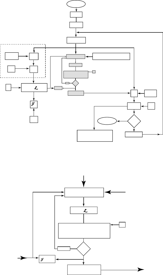
Figure 5.3.2 Generalized inversion of a regional quasigeostrophic model; indirect

representer algorithm.

Adjoint & Homogeneous

Forward Integration

(k)

= [δ

(k)

]

measurement

] ≡ 2b

-1

)

∇j

(k)

= P

-1

(k)

-1

= ∞

(∞)

(0)

= h

(k+1)

Adjoint & Forced

Forward Integration

preconditioner

rep coeffts

convergence

preconditioned

conjugate gradient solver

n-1

YES

k = k+1

priors

significance test

Figure 5.3.3 Data-space search engine.

148 5. The ocean and the atmosphere

(iii) The representer matrix should be tested for symmetry. The optimal values

β for

the representer coefﬁcients, found by the gradient solver, should be compared

to the values available a posteriori by measuring the inverse

u(x, t):

β =−˜w(L[

u] − d). (5.3.46)

(iv) Very large problems, such as those described in the following section, require

very powerful computers having massive memory and disk. It is difﬁcult to

offer further suggestions about implementations as each manufacturer provides

a unique software development environment. The results presented in this

chapter were obtained using Connection Machines.

(v) For pseudocode, code on ftp sites and extensive details for implementation see

Chua and Bennett (2001).

5.3.9

Track prediction

The intensity of tropical cyclones

is controlled by the thermodynamics of the atmos-

phere and ocean together. Predicting the intensity requires a fully stratiﬁed coupled

model. These are highly sensitive to the parameterization of heat exchange (Emanuel,

1999). Predicting the track of a typhoon, however, appears to be far simpler. The track

is largely determined by “steering” winds, taken to be either an average over the ﬁelds

in mid-troposphere, or else the ﬁelds at 500 mb. In either case, the evolution of these

winds can be represented for a short time (say, one-third of a synoptic time scale, or

about a day) by single-level, quasigeostrophic dynamics. These simpliﬁed dynamics

are nonetheless nonlinear, and so provide a relatively simple yet real and motivated ﬁrst

test for time-dependent variational assimilation in a nonlinear model. The formulation

has been discussed in some depth already, so only data need be discussed here. Further

details may be found in the ensuing references.

The state variable for the quasigeostrophic model (5.1.38) is the streamfunction

ψ = ψ(x, y, p, t); isobaric velocity u and vorticity ξ may be derived from it: see

(5.1.33), (5.1.34). Observations through the entire depth of atmosphere were col-

lected during a typhoon season by an international effort, the Tropical Cyclone ’90 or

TCM-90 experiment (Elsberry, 1990). These data were interpolated onto regular grids

by the Australian Bureau of Meteorology Research Centre (Davidson and McAvaney,

1981). The BMRC tropical analysis scheme uses a three-dimensional univariate stat-

istical interpolation method. Vortex centers were inserted manually and synthetic pro-

ﬁles were used to generate “observations” for the statistical analyses (Holland, 1980).

The gridded velocities were then partitioned into a rotational ﬁeld u

satisfy-

ing

k · ∇ × u

= 0, and a solenoidal ﬁeld u

satisfying ∇ · u

= 0. The gridded

streamfunction ψ for the latter ﬁeld became the data for the quasigeostrophic assim-

ilation. These streamfunction “data” were far from being direct measurements of the

Or typhoons, as they are known in the Paciﬁc (“hurricanes” in the Atlantic).

5.3 Tropical cyclones (1) 149

-24 24 48 (

)0-12

1100 1100 1100 1100 (GMT)2300

(8/28) (8/29) (8/30) (8/31) (1990)

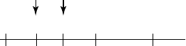
Figure 5.3.4 Time line for generalized

inversion of the tropical cyclone model.

Initial data are available at t =−24 in the

form of TCM-90 analyses. Boundary data

are available for −24 ≤ t ≤ 0, also from

TCM-90 analyses. For 0 ≤ t ≤ 48, the

boundary data are provided by a global

forecast of relatively coarse resolution. The

inverse takes advantage of additional

TCM-90 data, at t =−12 hours and at

t = 0 hours (as indicated by arrows). The

dates refer to TC “Abe”.

atmosphere. They were further modiﬁed by a projection onto the leading ten empirical

orthogonal functions (EOFs), which captured 94% of the variance. The time line for

these derived data, and for the assimilation-forecast episode is shown in Fig. 5.3.4. The

gridded streamfunction data at t =−24 hours constitute the prior initial condition, ten

EOF amplitudes were admitted at t =−12 and also at t = 0, and the smoothing or

inversion interval was −24 ≤ t ≤ 0. The gridded inverse streamfunction at time zero,

that is,

ψ(x, 0), became the initial condition for a forward integration or “forecast”

out to t =+48. The forecast was honest: boundary data for 0 ≤ t ≤ 48 were obtained

from a global forecast model also starting at t = 0, rather than from archived analyses.

Ten cases were considered; some involved the same typhoon in different stages of its

life. Detailed results may be found in Bennett et al. (1993).

From a scientiﬁc perspective the most interesting result is that the values of the

reduced penalty functional

J were broadly in the range 20 ± 6, as expected for χ

Thus the hypothesized error covariances were consistent with the data. A diagnosis

showed that the dynamical residuals and boundary vorticity residuals were negligible,

so it was the hypothesized error covariances for the initial conditions and data that were

consistent with the data.

From a control-theoretic perspective the most interesting result is that there were

sufﬁciently many degrees of freedom in the initial residuals at t =−24 to “aim” the

model at the few data, without additional “guidance” from dynamical residuals for

−24 ≤ t ≤ 0.

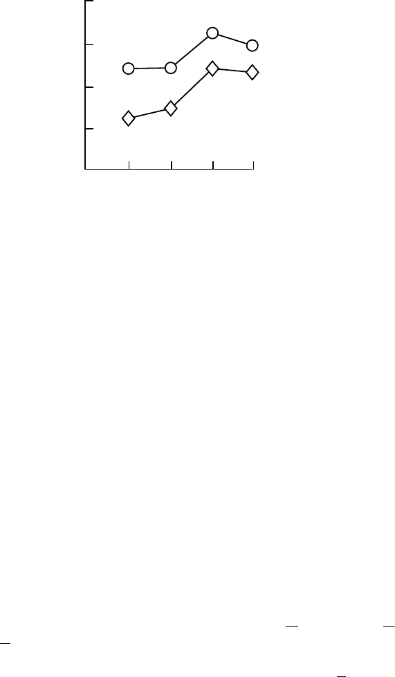
From a forecasting perspective the most interesting result was the skill enhance-

ment relative to other track prediction methods: see Fig. 5.3.5. Forty-eight-hour track

predictions based on variational assimilation over the preceding 24 hours were always

superior to those based on either a carefully tuned “nudging” scheme and/or a purely

statistical scheme (Bennett, Hagelberg and Leslie, 1992).

150 5. The ocean and the atmosphere

12 24 36 48

Hours

Improvement (%)

Figure 5.3.5 Tropical cyclone track

predictions. Percentage improvement in

(reduction of) mean forecast error to 48

hours ahead, relative to climatology plus

persistence (CLIPER). Diamonds: standard

initialization; circles: initialization by

generalized inversion. By convention the

7% difference at 48 hours, for example, is

scaled with respect to the 70% residual

yielding a “10% reduction”.

5.4 Tropical cyclones (2). Primitive Equations, intensity

prediction, array assessment

The evolution of a tropical cyclone is a thermodynamic process. Quasigeostrophic

dynamics assume that the stratiﬁcation remains close to the mean, and such is not the

case in a tropical cyclone. The Primitive Equations (see §5.1) include laws for:

(i) conservation of mass in a fully compressible gas, (5.1.9);

(ii) conservation of relative humidity q, (5.1.24);

(iii) conservation of entropy η, (5.1.24); and

(iv) an equation of state, (5.1.26), relating density ρ to η,toq and to the pressure p.

The state variable η may be replaced with the temperature T deﬁned by the com-

bined ﬁrst and second laws of thermodynamics:



∂η

∂T



= C

/T ,



∂η

∂T



= C

/T ,



∂η

∂v



= p/T , where v = ρ

−1

is the speciﬁc volume, while C

and C

are respec-

tively the speciﬁc heats at constant pressure and volume. For a dry, caloriﬁcally perfect

, C

constant) ideal (η = C

ln( pρ

−Cp/C

)) gas,

T = T





γ +1

η/C

. Empirical

corrections may be made for moisture: see, e.g., Wallace and Hobbs (1977).

Boltzmann’s equation leads directly to this deﬁnition of an ideal gas in terms of its entropy

dependence, rather than in terms of the gas law p = RρT . The latter merely deﬁnes

temperature. See, e.g., Chapman and Cowling (1970).

5.4 Tropical cyclones (2) 151

The full Primitive Equations may be found in Haltiner and Williams (1980, p. 17)

or in the appendix to Bennett, Chua and Leslie (1996, hereafter BCL1; the associated

Euler–Lagrange equations are also here in Appendix B). The vertical coordinate is

not simply the pressure p as in §5.1, but Phillip’s sigma-coordinate: σ = p/ p

∗

where

∗

is the pressure at the earth’s surface. The lower boundary for the atmosphere is

conveniently located at σ = 1.

A quadratic penalty functional for reconciling dynamics, initial conditions and data

is also given in BCL1, along with

(i) the nonlinear Euler–Lagrange equations;

(ii) the linearized Primitive Equations and Euler–Lagrange equations;

(iii) the representer equations and

(iv) the adjoint representer equations.

The linearized equations (ii)–(iv) enable an iterative solution of the nonlinear equa-

tions (i); each linear iterate may itself be solved by the indirect, iterative representer

method described in §3.1. The “inner” or “data space” search was preconditioned in

BCL1 using all representers calculated on a relatively coarse 128 × 64 × 9 global grid

with two-minute time steps, see Bennett, Chua and Leslie (1997, hereafter BCL2).

The smallness of the time steps is due to the polar convergence of the meridians. The

inverse was calculated on a relatively ﬁne 256 × 128 × 9 global grid with one-minute

time steps. There were 4.4 × 10

grid points in a twenty-four-hour smoothing interval,

for about 2.6 × 10

gridded values of u, v,˙σ , T , q,lnp

∗

, etc.

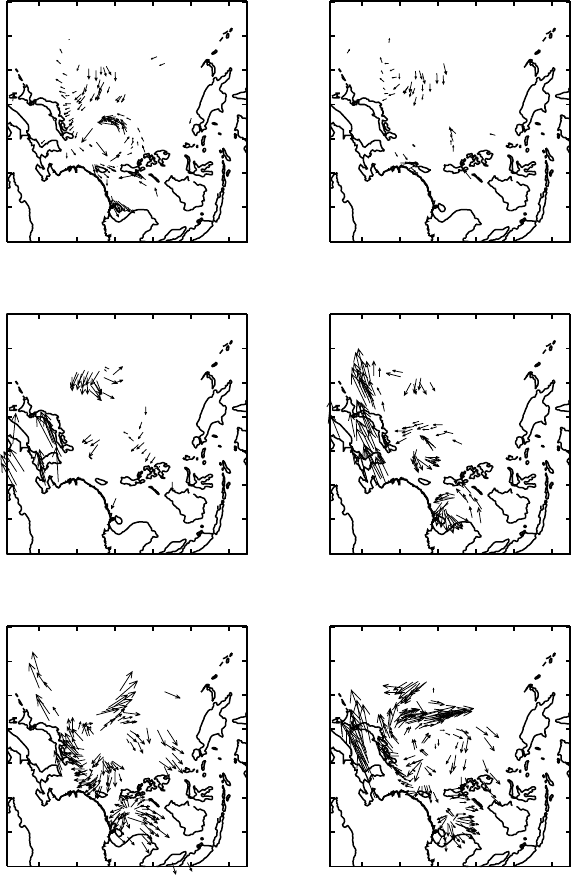
The coarse-grid preconditioner was only moderately effective owing to errors of

interpolation from the coarse grid to the data sites. The latter were reprocessed cloud

track wind observations (RCTWO) inferred from consecutive satellite images of middle

and upper-level clouds (Velden et al., 1992). Some of these observations are shown

in Fig. 5.4.1. The observation period included tropical cyclone “Ed” near (113

◦

N) and Supertyphoon

“Flo” near (130

◦

E, 23

◦

N). The RCTWO were available

at t =−24, −18, −12 and 0 hours, and at 850 hPa, 300 hPa and 200 hPa for a total

of M = 2436 vector components. The measurement errors for each component were

assumed to be 3 m s

−1

,4ms

−1

and4ms

−1

at the respective levels, uncorrelated from

the other component of the same vector and from all other vectors elsewhere and at

different times. The single inversion reported in BCL1 reduced the penalty functional

from a prior value of 6432 to a posterior value of 4066. It may be concluded that the

forward model and initial conditions (an ECMWF analysis) were very good, that the

RCTWO only had moderate impact, and that the prior root mean square error should

have been 30% larger. Given the difﬁculty in estimating the dynamical errors, such a

conclusion is incontestable. Assimilation of the RCTWO did however have a useful

impact on subsequent forecasts of meridional wind ﬁelds near “Flo”: see BCL1. Of

greater interest here are the representers, for the Primitive Equation dynamics linearized

According to the Japanese Meteorological Agency.

110E 130E 150E 170E

200 hPa

10S

10N

20N

30N

40N

(t=-12)

110E 130E 150E 170E

300 hPa

10S

10N

20N

30N

40N

110E 130E 150E 170E

850 hPa

10S

10N

20N

30N

40N

110E 130E 150E 170E

200 hPa

10S

10N

20N

30N

40N

(t=0)

110E 130E 150E 170E

300 hPa

10S

10N

20N

30N

40N

110E 130E 150E 170E

850 hPa

10S

10N

20N

30N

40N

Figure 5.4.1 Reprocessed cloud track wind observation vectors at 200 hPa, 300 hPa and 850 hPa, at t =−12 or 0000UTC on 16/IX/1990

(upper panels), and at t = 0 or 0000UTC on 16/XI/1990 (lower panels). RCTWO data are also available at t =−24, and at t =−18, for a

total of 2436 scalar data (after Bennett, Chua and Leslie, 1996).

5.4 Tropical cyclones (2) 153

-1

0 60E 120E 180 120W 60W

60S

30S

30N

60N

-1

0 60E 120E 180 120W 60W

60S

30S

30N

60N

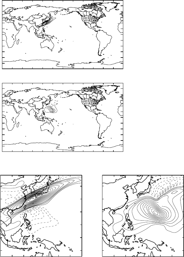
Figure 5.4.2 Zonal velocity

ﬁelds at ( p = 200 hPa,

t = 0) for representers of

two RCTWO zonal

components also at (200,0).

Units are m

−2

,asfor

velocity autocovariances

(after Bennett, Chua and

Leslie, 1997).

0.75

-0

-0.25

-1.00

1.50

3.00

6.00

-0.25

-1.00

110E 130E 150E 170E

10S

10N

20N

30N

40N

-0.25

-0

.25

-1.00

0.75

1.50

3.00

110E 130E 150E 170E

10S

10N

20N

30N

40N

Figure 5.4.3 As for Fig. 5.4.2; close-ups over the S. China Sea (after Bennett, Chua

and Leslie, 1997).

about the ﬁfth and ﬁnal “outer” iterate of the inverse estimate. Upper level zonal winds

for two representers are shown in Fig. 5.4.2, and in close-up in Fig. 5.4.3. Their striking

anisotropy is a consequence of shearing by supertyphoon winds. The eigenvalues of

the M × M representer matrix R and its stabilized form P = R + C



, where C



154 5. The ocean and the atmosphere

110E 130E 150E 170E

200 hPa

10S

10N

20N

30N

40N

(T=-12)

110E 130E 150E 170E

300 hPa

10S

10N

20N

30N

40N

110E 130E 150E 170E

850 hPa

10S

10N

20N

30N

40N

110E 130E 150E 170E

200 hPa

10S

10N

20N

30N

40N

(T=0)

110E 130E 150E 170E

300 hPa

10S

10N

20N

30N

40N

110E 130E 150E 170E

850 hPa

10S

10N

20N

30N

40N

110E 130E 150E 170E

200 hPa

10S

10N

20N

30N

40N

(T=-24)

110E 130E 150E 170E

300 hPa

10S

10N

20N

30N

40N

110E 130E 150E 170E

850 hPa

10S

10N

20N

30N

40N

110E 130E 150E 170E

200 hPa

10S

10N

20N

30N

40N

(T=-18)

110E 130E 150E 170E

300 hPa

10S

10N

20N

30N

40N

110E 130E 150E 170E

850 hPa

10S

10N

20N

30N

40N

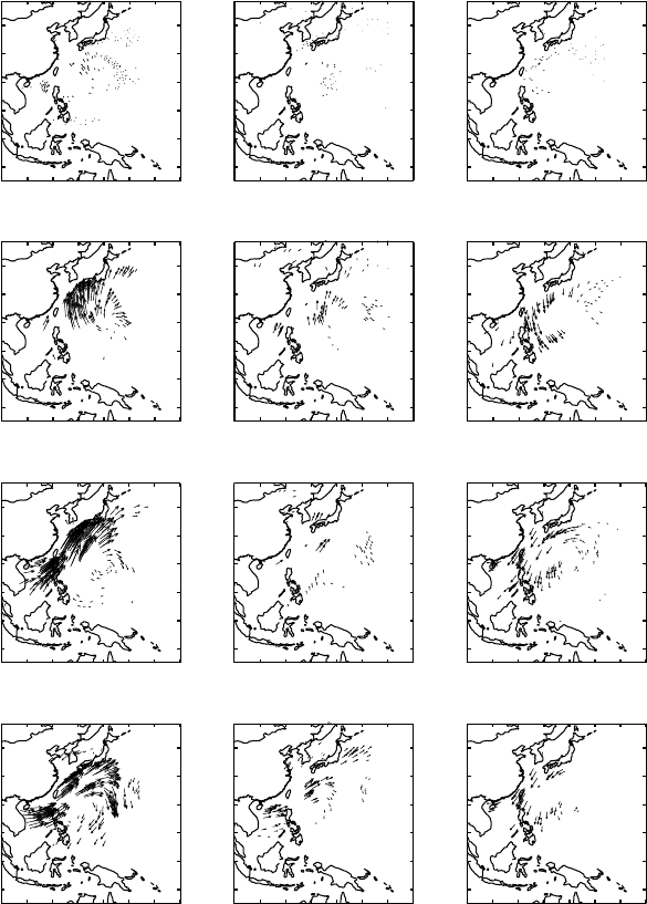
Figure 5.4.4a The ﬁrst orthonormalized eigenvector z

of the symmetric

positive-deﬁnite matrix P = R + C



the data error covariance matrix, may be seen in BCL1. Recall that R was calculated

on the relatively coarse grid as a preconditioner for indirect inversion on the ﬁne grid.

Given the assumed levels of data error, there are only about 200 effective degrees of

freedom in the observations. Thus only about 200 iterations would be needed in order

to solve (3.1.6). The coarse grid precondition reduced the number to below 15.

The ﬁrst and fourth leading normalized eigenvectors of P are shown in Fig. 5.4.4.

They are associated with the ﬁrst and fourth largest eigenvalue of P: see §2.5 and

5.4 Tropical cyclones (2) 155

110E 130E 150E 170E

200 hPa

10S

10N

20N

30N

40N

(T=-24)

110E 130E 150E 170E

300 hPa

10S

10N

20N

30N

40N

110E 130E 150E 170E

850 hPa

10S

10N

20N

30N

40N

110E 130E 150E 170E

200 hPa

10S

10N

20N

30N

40N

(T=-18)

110E 130E 150E 170E

300 hPa

10S

10N

20N

30N

40N

110E 130E 150E 170E

850 hPa

10S

10N

20N

30N

40N

110E 130E 150E 170E

200 hPa

10S

10N

20N

30N

40N

(T=-12)

110E 130E 150E 170E

300 hPa

10S

10N

20N

30N

40N

110E 130E 150E 170E

850 hPa

10S

10N

20N

30N

40N

110E 130E 150E 170E

200 hPa

10S

10N

20N

30N

40N

(T=0)

110E 130E 150E 170E

300 hPa

10S

10N

20N

30N

40N

110E 130E 150E 170E

850 hPa

10S

10N

20N

30N

40N

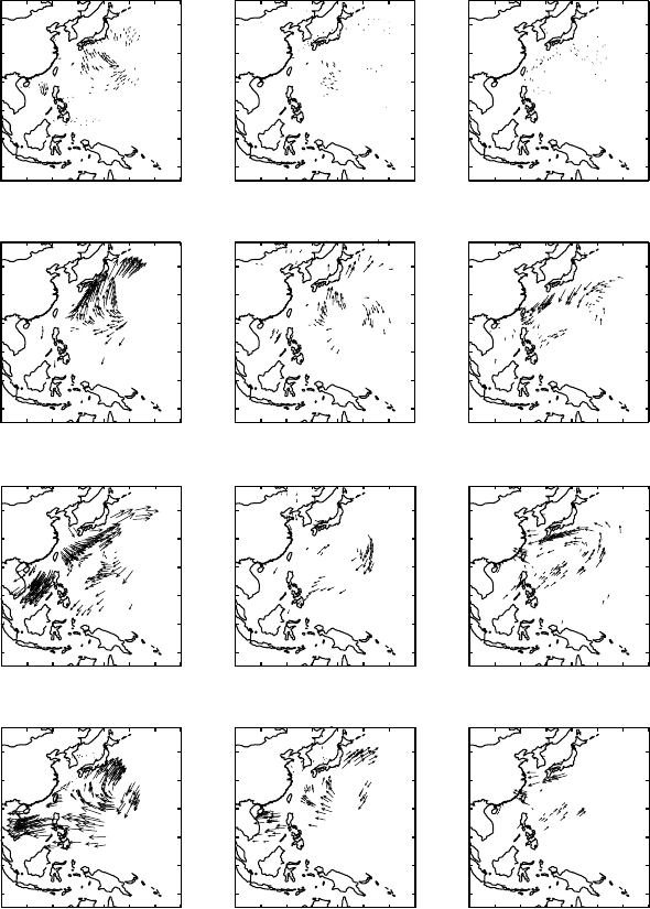
Figure 5.4.4b The fourth eigenvector z

especially (2.5.4). These are the ﬁrst and fourth most stably observed wind patterns.

There is cross-correlation between wind components u and v; there is autocorrelation in

time and there is autocorrelation in height. The amplitudes of the winds are asymmetric

with respect to the centers of the tropical cyclones, evidently as a consequence of

strongly asymmetrical advection. The two eigenvectors display markedly different

ﬂow topologies. Variational methods are capable of extracting non-intuitive covariance

structure from dynamics, even if the use of such methods for actual assimilation or

analysis cannot be afforded in real time. The real-time imperative is most demanding

156 5. The ocean and the atmosphere

in numerical weather prediction, but is far less demanding in seasonal-to-interannual

climate prediction.

5.5

ENSO: testing intermediate coupled models

The Tropical Atmosphere–Ocean array developed for the Tropical Ocean–Global

Atmosphere experiment, or TOGA-TAO array, is providing an unprecedented in situ

data stream for real-time monitoring of tropical Paciﬁc winds, sea surface temper-

ature, thermocline depths and upper ocean currents. For a tour of the project, and

for data display and distribution, see www.pmel.noaa.gov/tao/home.html. The

data are of sufﬁcient accuracy and resolution to allow for a coherent description of

the basin scale evolution of these key oceanographic variables. They are critical for

improved detection, understanding and prediction of seasonal to interannual climate

variations originating in the Tropics, most notably those related to the El Ni˜no Southern

Oscillation (ENSO) (McPhaden, 1993, 1999a,b). The freely-distributed TAO display

software provides gridded SST and 20

◦

isotherm depth (Z20) using an objective analy-

sis procedure. The ﬁrst-guess ﬁelds are those of Reynolds and Smith (1995) for SST;

a combination of Kessler (1990) expendable bathythermograph (XBT) analyses and

Kessler and McCreary (1993) conductivity, temperature, and depth analyses for Z20,

and Comprehensive Ocean–Atmosphere Data Set analyses (Woodruff et al., 1987) for

surface winds. The procedure is univariate and involves bilinear interpolation followed

by smoothing with a gappy running mean ﬁlter (Soreide et al., 1996).

Given this splendid and growing data set (see the TOGA-TAO website), the question

arises: can it be better analyzed by generalized inverse methods? That is, can it be

better interpolated, or more generally smoothed using a dynamical model as a guide?

The question is addressed by Kleeman et al. (1995) who vary the initial conditions

and parameters of an “intermediate” coupled model. Miller et al. (1995) apply the

Kalman ﬁlter to a linear intermediate ocean model expanded in its natural Rossby

wave modes; dynamical errors or “system noise” are admitted and these are assumed

to be uncorrelated in time or “white”.

Bennett et al. (1998, 2000, hereafter BI, BII) seek upper ocean ﬁelds and lower

atmosphere ﬁelds that provide weighted, least-squares best-ﬁts to 12 and 18 month

segments of monthly mean TAO data, and to a nonlinear intermediate coupled model

after that of Zebiak and Cane (1987). The model structure is indicated schematically

in Fig. 5.5.1; the equations of motion may be found in the references. The dynami-

cal variables are anomalies of current, wind temperature and layer thickness, relative

to their respective annual cycles. The oceanic and atmospheric dynamics are linear,

save for the presence of anomalous advection of anomalous heat in the oceanic upper

layer, for the quadratic dependence of anomalous surface stress upon anomalous wind,

and for the parameterization of turbulent vertical mixing in the ocean in terms of a