Bennett A.F. Inverse Modeling of the Ocean and Atmosphere

Подождите немного. Документ загружается.

5.2 Ocean tides 137

0 50 100 150 200 250 300 350

⫺60

⫺40

⫺20

⫺25 ⫺20 ⫺15 ⫺10 ⫺50

W/m

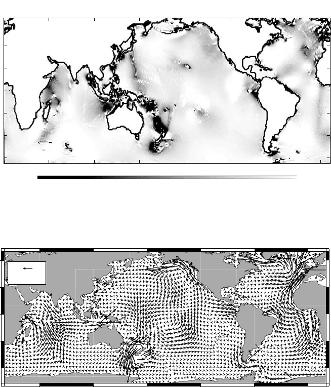
Figure 5.2.7 Per-cycle average rate of working of the M

dynamical residuals in

TPX0.4 on the M

tide, in units of W m

−2

.Negative values indicate that the M

tide

is losing energy (after Egbert, 1997).

60˚ 120˚ 180˚ 120˚ 60˚ 0˚

60˚

30˚

0˚

30˚

60˚

200 kW/m

Figure 5.2.8 Flux of total mechanical energy for the linear semidiurnal tidal

constituent M

, based on the inverse model TPX0.4. Note especially the convergence

into regions of signiﬁcant tidal dissipation: for example, the North West Australian

shelf, Micronesia/Melanesia and the European shelf (Egbert and Ray, 2001:

Estimates of M

tidal energy dissipation from TOPEX/POSEIDON altimeter data,

J. Geophys. Res.,inpress.

 2001 American Geophysical Union, reproduced by

permission of American Geophysical Union).

The various highly accurate tidal solutions are leading to reﬁned estimates of the

dissipation of the energy input to the ocean by the tide-generating force (Lyard and

Le Provost, 1997; Le Provost and Lyard, 1997; Egbert and Ray, 2000, 2001). These

estimates show that tidal dissipation can provide about 50% of the 2TW of power

believed to sustain the meridional overturning circulation, the other 50% being provided

by the wind (Wunsch, 1998). A map of energy ﬂux vectors for the tides is shown in

Fig. 5.2.8. Some of this power is being produced by the dynamical residuals. Note

138 5. The ocean and the atmosphere

that there are strong convergences and divergences in deep water, as well as ﬂuxes

towards the marginal seas. These deepwater convergences and divergences almost

exactly balance the work done by the moon.

5.3

Tropical cyclones (1). Quasigeostrophy;

track predictions

5.3.1 Generalized inversion of a quasigeostrophic model

The linear “toy” ocean model of §1.1 and the linear Laplace Tidal Equations of §5.2 are

not representative of ocean circulation, which has nonlinear dynamics and thermo-

dynamics. The generalized inverse of a nonlinear quasigeostrophic model is now

deﬁned and the Euler–Lagrange equations are derived. The latter equations are also

nonlinear, so the linear representer algorithm can only be applied iteratively. Two

iteration schemes are introduced; a more extensive analysis is provided in §3.3.3. The

formulation of an hypothesis for the dynamical errors, which difﬁcult subject was

broached §5.2, is considered further here. Finally, implementation of the representer

algorithm is discussed in some detail.

5.3.2

Weak vorticity equation, a penalty functional,

the Euler–Lagrange equations

Let us formulate weak quasigeostrophic dynamics entirely in terms of the stream-

function ψ:

∂

∂t

∇

ψ +

∂(ψ, ∇

ψ + f )

∂(x, y)

= τ, (5.3.1)

where τ is the residual in the quasigeostrophic vorticity equation. We shall also specify

a weak initial condition for ψ:

ψ(x, 0) = ψ

(x) + i (x), (5.3.2)

where i is the initial residual. A weak condition for ψ on the boundary B of the

simply-connected domain D is

ψ(x, t ) = ψ

(x, t) + b(x, t), (5.3.3)

where x lies on B, and b is the boundary streamfunction residual. We shall weakly

specify the relative vorticity all around B:

∇

ψ(x, t ) = ξ

(x, t) + z(x, t), (5.3.4)

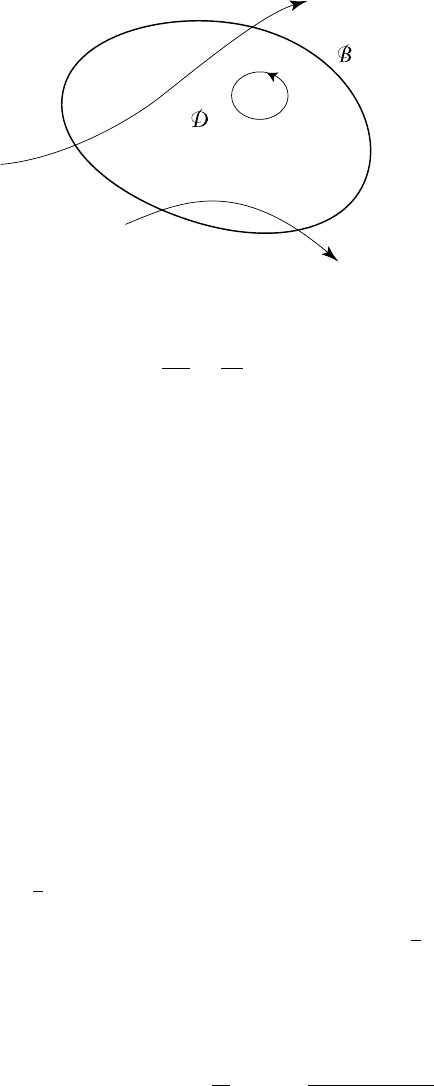
where x lies on B and z is the boundary vorticity residual. See Fig. 5.3.1.

5.3 Tropical cyclones (1) 139

Figure 5.3.1 Planar domain

D with open boundary B.

Streamlines cross B at least

twice, or not at all. What can

be said about particle paths?

Now (5.3.1) is equivalent to

Dζ

∂ζ

∂t

+ u · ∇ζ = τ, (5.3.5)

where ζ ≡∇

ψ + f . It follows that if τ is prescribed, then ζ is determined by inte-

grating (5.3.5) along a particle path from an initial position either inside D or on the

boundary B. If any particle path exits D in the time interval of interest, then (5.3.4)

overdetermines ζ . However we shall “adjust” the residuals τ , i, b and z, so that a con-

tinuous solution is obtained for ζ , and hence for ψ. More precisely, we shall seek ψ

yielding a smooth weighted-least-squares best-ﬁt to (5.3.1)–(5.3.4). A suitable penalty

functional is (Bennett and Thorburn, 1992):

J [ψ ] = τ • C

−1

• τ + i ◦ C

−1

◦ i + b ∗ C

−1

∗ b + z ∗ C

−1

∗ z + J

, (5.3.6)

where J

is a penalty for misﬁts to data within D. Note that

•≡





dt da, ◦=



da, ∗=



dt ds, (5.3.7)

and all integrations are on a surface of constant pressure p.If

ψ is a local extremum

of J , then

δJ [

ψ] = δτ • C

−1

• ˆτ + δψ ◦ C

−1

◦

+δψ ∗ C

−1

∗

b + δξ ∗ C

−1

∗

z +

δJ

= 0. (5.3.8)

We shall manipulate the ﬁrst two terms in detail, leaving the boundaries as an exercise.

Deﬁne

λ ≡ C

−1

• ˆτ . Then

δτ •

λ =





dt da



∂

∂t

∇

ψ + δ

∂(ψ, ∇

ψ + f )

∂(x, y)



λ(x, t). (5.3.9)

140 5. The ocean and the atmosphere

The ﬁrst term in (5.3.9) is easily manipulated:



∂

∂t

∇



λ =



∂

∂t

∇

δψ



∂

∂t

(

λ∇

δψ) −



∂

∂t



∇

δψ. (5.3.10)

Integrating the ﬁrst term in (5.3.10) over time yields

[

λ∇

δψ]

t=0

. (5.3.11)

Now

λ∇

δψ = ∇ · (

λ∇δψ − δψ∇

λ) + δψ∇

λ. (5.3.12)

If the area integral of terms proportional to δψ(x, T ) vanishes, for arbitrary values of

the latter, then

∇

λ = 0att = T. (5.3.13)

Similarly, we infer that

−∇

λ + C

−1

◦ (

ψ − ψ

) = 0att = 0. (5.3.14)

The second term in (5.3.10) is

−



∂

∂t



∇

δψ =−∇ ·



∂

∂t

∇δψ − δψ∇

∂

∂t



− δψ∇

∂

∂t

. (5.3.15)

The second term in (5.3.15) will be used shortly. Consider now the variation of the

Jacobian in (5.3.9):

λδ

∂(ψ, ∇

ψ + f )

∂(x, y)

∂(δψ, ∇

ψ + f )

∂(x, y)

∂(

ψ,δ∇

ψ)

∂(x, y)

+ O(

λ(δψ)

) (5.3.16)

... =−δψ



∂(

λ, ∇

ψ + f )

∂(x, y)

+∇

∂(

λ,

ψ)

∂(x, y)

+divergence terms. (5.3.17)

So, by requiring the coefﬁcient of δψ(x, t) to vanish, we recover from (5.3.8), (5.3.15)

and (5.3.17) the Euler–Lagrange equation

−

∂

∂t

∇

λ −∇

∂(

ψ,

λ)

∂(x, y)

∂(

λ, ∇

ψ + f )

∂(x, y)

−

δJ

δψ

, (5.3.18)

where the last term is a linear combination of measurement kernels. Equation (5.3.18)

may be formally rewritten as

−

∂

∂t

− ∇ · (

λ) =∇

−2

ˆµ · ∇

ζ −

∇

−2



δJ

δψ



, (5.3.19)

5.3 Tropical cyclones (1) 141

where

u =



−

∂

∂y

∂

∂x



and ˆµ ≡



−

∂

∂y

∂

∂x



. Note that ∇ ·

u = ∇ · ˆµ = 0. The form

(5.3.19) looks like the “adjoint” of the total vorticity conservation law

∂ζ

∂t

+ u · ∇ζ = τ, (5.3.20)

but for the emergence of a new term on the rhs of (5.3.19) arising from the variation of

the advecting velocity u:

δτ =

∂

∂t

δζ + u · ∇δζ + (δu) · ∇ ζ. (5.3.21)

No such term arose in our “toy” model

∂u

∂t

+ c

∂u

∂x

= τ , since the phase velocity c was

ﬁxed. In particular c did not depend upon the state u.

Exercise 5.3.1

Derive the boundary conditions that accompany the variational equation (5.3.18)

or (5.3.19). Which boundary condition goes with which equation? 

5.3.3

Iteration schemes; linear Euler–Lagrange equations

The Euler–Lagrange system (5.3.1) and (5.3.18), with attendant initial and boundary

conditions, is nonlinear. The system is coupled through the data term (δJ

/δψ)in

(5.3.18), through advection on the lhs of (5.3.18) and through the other term on the

rhs of (5.3.18). It is also coupled through the boundary conditions. A simple iteration

scheme breaks the coupling completely: calculate a sequence {

,λ

}

∞

n=1

such that

∂

∂t

∇

∂(

, ∇

+ f )

∂(x, y)

= C

• λ

, (5.3.22)

−

∂

∂t

∇

−∇

∂(

n−1

,λ

)

∂(x, y)

∂(λ

n−1

, ∇

n−1

+ f )

∂(x, y)

−

δJ

n−1

δψ

. (5.3.23)

These equations may be solved by integrating (5.3.23) backwards, and (5.3.22) for-

wards. Note that (5.3.22) is nonlinear in

, but the broken coupling eliminates the

need for representers! However, such a sequence always seems to diverge.

An alternative iteration scheme is:

∂

∂t

∇

∂(

n−1

, ∇

+ f )

∂(x, y)

= C

• λ

, (5.3.24)

−

∂

∂t

∇

−∇

∂(

n−1

,λ

)

∂(x, y)

∂(λ

n−1

, ∇

n−1

+ f )

∂(x, y)

−

δJ

δψ

. (5.3.25)

This system is linear, but coupled: note that the data term in (5.3.25) is evaluated with

. It is the Euler–Lagrange system for a linear dynamical model, advected by

n−1

There is a ﬁrst-guess forcing C

• λ

, where λ

is the response of the lhs of (5.3.25) to

the ﬁrst term on the rhs. The system may be solved using representers. The sequence

142 5. The ocean and the atmosphere

converges in practice if the Rossby number is moderate. There are some theorems

about convergence in doubly-periodic domains: the sequence is bounded and so must

have points of accumulation or cluster points, but not necessarily unique limits. There

is numerical evidence of the sequence cycling, presumably between cluster points. A

third iteration scheme is described in §3.3.3.

5.3.4

What we can learn from formulating

a quasigeostrophic inverse problem

A quasigeostrophic inverse model offers some especially clear problems in error esti-

mation. Also, there are special opportunities for reliable estimation of these errors. To

the extent that the situation is not representative of Primitive Equation inverse models,

one might regard quasigeostrophic inversion as a curiosity but, like the uniquely elegant

tidal inverse problem, the quasigeostrophic inverse problem offers valuable experience.

5.3.5

Geopotential and velocity as streamfunction data:

errors of interpretation

There are errors of interpretation in certain streamfunction data. Consider geopotentials

φ and horizontal velocities u measured by radar-tracking of high altitude balloons, or

by sonar-tracking of deeply submerged ﬂoats. The quasigeostrophic state variable is the

streamfunction ﬁeld ψ. We must relate φ and u to ψ . The geostrophic approximation is

k × u

∼

−∇φ, (5.3.26)

where the Coriolis parameter is a function of latitude: f = f (y). We have assumed

that ∇ · u

∼

0 and that there is a streamfunction for ψ, so (5.3.26) becomes

− f ∇ψ

∼

−∇φ. (5.3.27)

Ignoring variations in f leads to the “poor man’s balance equation”

ψ = φ, (5.3.28)

where f

= f (y

) for some latitude y

. Hence geopotential data may be used as

approximations to streamfunction data. Also, velocity data may be used as approxi-

mations to streamfunction-gradient data:

∇ψ =−

k × u. (5.3.29)

Let us begin to estimate the errors in (5.3.28) and (5.3.29). If L is a horizontal length

scale and U is a velocity scale, then the local acceleration neglected in (5.3.26) has the

scale U

−1

. The Coriolis acceleration retained in (5.3.26) has the scale f

U , so the

relative errors in (5.3.26) scale as the Rossby number Ro ≡

. We shall assume for

5.3 Tropical cyclones (1) 143

simplicity that variations in f are smaller than Rof

. Then (5.3.26) is

k × u =−f

−1

∇φ + O(URo), (5.3.30)

hence

∇ · u = O





. (5.3.31)

In general, for any u there is a streamfunction ψ and a velocity potential χ such that

u =

k × ∇ψ + ∇χ ≡ u

+ u

, (5.3.32)

thus

ξ ≡

k · ∇ × u =∇

ψ, δ ≡ ∇ · u =∇

χ. (5.3.33)

We conclude from (5.3.31) that χ is O(Ro U L) and hence (5.3.29) is accurate to

O(Ro U), while (5.3.28) is accurate to O(Ro f

UL). In summary, the “theoretical”

relative errors in the data are O(Ro), where Ro ≡ U/( f

L). For Gulf Stream meanders

in the ocean, U = 1ms

−1

(=2 knots), L = 10

m and f

= 10

−4

−1

,soRo = 0.1.

For middle-level synoptic-scale weather systems in the atmosphere, U = 30 m s

−1

and

L = 10

m, so Ro = 0.3.

In the preceding analysis, the estimates of neglected local accelerations were based

on the values L and U representative of the synoptic-scale circulation of interest.

For consistency, all ﬁelds should be low-pass ﬁltered prior to sampling, in order to

suppress smaller-scale motions such as internal waves. If, as is often unavoidable,

the smoothing is inadequate, then the data will be contaminated with aliased signals.

This contamination can be substantial, exceeding for example the estimate O(RoU)

for errors in (5.3.29). (I am grateful to Dr Ichiro Fukumori for a discussion of this

point. AFB)

5.3.6

Errors in quasigeostrophic dynamics: divergent ﬂow

Estimating the dynamical errors in a quasigeostrophic model is particularly instruc-

tive, as we have closed analytical forms for many sources of error. Recall again the

momentum balance for the Primitive Equations:

∂u

∂t

+ (u · ∇)u + ω

∂

∂p

u + f

k × u =−∇φ. (5.3.34)

Taking the curl at constant pressure yields

∂ξ

∂t

+ (u · ∇)ξ + ω

∂ξ

∂p

k · ∇ω ×

∂u

∂p

+ ( f + ξ)δ + βv = 0, (5.3.35)

144 5. The ocean and the atmosphere

where ξ =

k · ∇ × u, δ = ∇ · u and β ≡ df/dy. Splitting u into a solenoidal part u

and an irrotational part u

(see (5.3.31)) leads to a split for (5.3.35):

∂ξ

∂t

+(u

·∇)ξ +βv

=−(u

·∇)ξ −( f +ξ )δ −βv

−ω

∂ξ

∂p

−

k ·∇ ω ×

∂u

∂p

≡τ.

(5.3.36)

That is,

∂

∂t

∇

ψ +

∂(ψ, ∇

ψ + f )

∂(x, y)

= τ, (5.3.37)

where we have an explicit form for τ in terms of resolvable ﬁelds. That is, given archives

of gridded ﬁelds of u(x, p, t), we may evaluate τ on the grid, and hence estimate its

mean E τ and covariance C

. The most difﬁcult part is calculating ω reliably. We could

use the conservation of mass:

∂ω

∂p

=−∇ · u, (5.3.38)

subject to ω → 0as p → 0, or we could use the conservation of entropy:

ω =



−

∂η

∂t

− u · ∇η



∂η

∂p



−1

, (5.3.39)

where

Q is the heat source per unit mass and T is the absolute temperature. Note that in

order to calculate η and T via the equation of state, we need the other thermodynamic

state variables such as ( p,ρ,q) in the atmosphere, or ( p,ρ,S) in the ocean. We may

dispense with ρ if T has been measured or is otherwise available on the grid.

There are opportunities to make similar direct estimates of dynamical errors in other

“reduced” models, such as balanced models, and the Cane–Zebiak coupled model

(Zebiak and Cane, 1987). However, there are additional dynamical errors in all these

reduced models, owing to unresolved stresses. The additional errors may exceed the

resolvable errors.

5.3.7

Errors in quasigeostrophic dynamics:

subgridscale ﬂow, second randomization

We shall consider the unresolved stresses, in the context of the quasigeostrophic vor-

ticity equation

∂ξ

∂t

+ u · ∇ξ + βv = 0, (5.3.40)

where ξ =∇

ψ and u =

k × ∇ψ. Note that the subscript “ψ”onu is now dropped. In

practice we can only calculate with (5.3.40) on a grid having some ﬁnite resolution in

space and time. Yet we know from observations and from instability theory that (5.3.40)

possesses solutions that have inﬁnitesimally ﬁne structure of signiﬁcant amplitude.

5.3 Tropical cyclones (1) 145

We try to separate the coarse and ﬁne structures using the abstraction of an ensemble

of ﬂows having a mean (with only the coarse scales), and variability (with only the ﬁne

scales). That is, ξ =

ξ + ξ



, where ξ = ξ and ξ



= 0. In practice we can only approxi-

mate the ensemble average (denoted by

( ) here) using a space or time average



(),but

then (



ξ) =

ξ. We shall ignore this very important issue here (see Ferziger, 1996 for

an excellent discussion) and assume that

( ) may be estimated with adequate accuracy.

Only the mean ﬁeld being of interest, it would be desirable to replace the “detailed”

vorticity equation (5.3.40) with an equation for

ξ,u and ψ. Averaging (5.3.40) yields

∂

∂t

ξ + u · ∇ξ + βv = 0. (5.3.41)

Now for any a and b,

ab = (a + a



)(b + b



)

(ab + ab



+ a



b + a



)

a b + a b



+ a



b + a



(!)

ab + a0 +0b + a



= ab + a



(5.3.42)

Thus

u · ∇ξ = u · ∇ξ + u



· ∇ξ



(5.3.43)

and (5.3.41) becomes

∂

∂t

u · ∇ξ + βv = τ ≡−∇ · (u



), (5.3.44)

where we have used ∇ · u



= 0. So there is another candidate for the residual τ in the

mean dynamics: the divergence of the mean “eddy-ﬂux” of relative vorticity. Finding

a formula for such ﬂuxes in terms of ﬁrst moments (that is, in terms of

ξ, u or ψ) is the

turbulence problem. It remains unresolved. However, we may use (5.3.44) to constrain

the circulation, provided we can put bounds on

τ . At this point the fast talk begins.

Realizing that even the smoothed ﬁelds ﬂuctuate considerably, we may regard

τ as a

random ﬁeld with a prior mean and variance (prior to assimilating data). Generally we

neglect the new mean E

τ for τ (or else model it with a diffusion law, for example),

and struggle to make scale estimates for the variability in

τ . For example, if for the

eddies |

u|∼U and |x|∼l, we might be tempted to assume τ ∼ U

−2

. This is usually

excessive; the length scale L of the (smoothed) eddy-ﬂux



is much greater than the

length scale l of the eddies themselves. That is,

τ ∼ cU

−1

, where c 1isthe

magnitude of the correlation coefﬁcient between u



and ξ



. The decorrelation length

scale D for

τ presumably lies in the interval l < D < L, while the decorrelation time T

lies in the range (l/U) < T < (L/U). In the jet stream or ocean boundary currents, on

146 5. The ocean and the atmosphere

the other hand, l ∼ L. For the weakly homogeneous case (l  L), however, we might

hypothesize that

τ (x, t)τ (y, s)) = C

(x, t, y, s) =

exp



−

|x − y|

−

|t − s|



. (5.3.45)

One might reasonably feel uncomfortable at this point, attempting to constrain a circu-

lation estimate with such a speculative hypothesis. Indeed, the “second randomization”

τ isana¨ıve abstraction of the hoped-for scale separations in the ﬂuctuations in τ .

One should recall that the conventional forward model is merely a circulation estimate

based on the hypothesis that

τ ≡ 0. This is the one hypothesis that we know immedi-

ately to be wrong. We could abandon the concept of an ensemble of mean vorticity

ﬂuxes, and just manipulate

τ as a control that guides the state towards the data. The

Euler–Lagrange equations of the calculus of variations enable the manipulations, once

a penalty functional has been prescribed. The difﬁculty lies in the choice of weights.

Probabilistic choices (inverses of covariances) are conceptually shaky. Yet the prospect

of an ocean model as a testable hypothesis is so appealing.

It was established in §2.2 that generalized inversion is equivalent to optimal interp-

olation in space and time. The former requires the dynamical error covariance C

;

the latter requires the circulation or state covariance such as C

. Which is the easier

to specify a priori? We anticipate that ψ is nonstationary, anisotropic and signiﬁcantly

inhomogeneous. The components of multivariate circulation ﬁelds will be jointly co-

varying. On the other hand, it is plausible that the dynamical residuals in unreduced

models are the result of small-scale processes that are locally stationary, isotropic and

univariate. Then the generalized inverse constructs highly structured state covariances

guided by the model dynamics, and by the morphology of the domain: the orography,

or the bathymetry and coastline.

5.3.8

Implementation; ﬂow charts

The linear representer method is complicated. Its iterative application to a nonlinear

quasigeostrophic model makes it even more complicated. Some general suggestions

on implementation are in order.

(i) Start with a simple, linear problem ﬁrst, such as the one described in §1.1–§1.3.

The computing exercises at the end of this book provide numerical details.

FORTRAN code is available from an anonymous ftp site:

ftp.oce.orst.edu, cd/dist/bennett/class.

(ii) A ﬂow chart for the “quasigeostrophic inverse” is given in Figs. 5.3.2 and 5.3.3.

The latter ﬁgure shows in detail the hatched section in the former. These

computations are manageable using a workstation. Your code should consist of

a main program that calls many subroutines. These should include a single

“backward integration” and a single “forward integration”. Preconditioned

conjugate gradient solvers are widely available in subroutine libraries.