Bennett A.F. Inverse Modeling of the Ocean and Atmosphere

Подождите немного. Документ загружается.

5.5 ENSO: testing intermediate coupled models 157

(1)

(2)

(1)

+θ

(1)

(2)

+θ

(2)

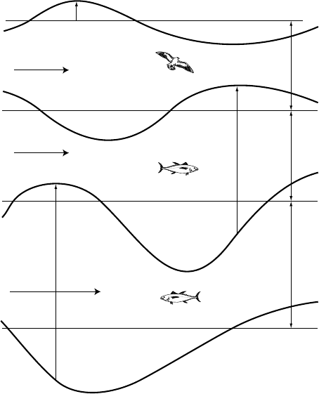
Figure 5.5.1 A reduced

gravity, two-and-one-half

layer ocean model coupled

to a reduced gravity,

one-and-one-half layer

atmospheric model (after

Bennett et al., 1998).

piecewise differentiable switching function. The ocean model domain is a rectangle

on the equatorial beta plane: (123.7

◦

E, 84.5

◦

W) × (29

◦

S, 29

◦

N). The atmospheric

model domain is an entire equatorial zone (29

◦

S, 29

◦

N). The inclusion of local ac-

celerations in all the momentum equations permits the satisfaction of rigid meridional

boundary conditions in the ocean, and the satisfaction of rigid zonal boundary con-

ditions in both the ocean and atmosphere. The inclusion of pseudoviscous stresses

permits the satisfaction of no slip and free slip at meridional and zonal boundaries

respectively.

The generalized inverse of this intermediate coupled model and the TAO data is,

again, the weighted least-squares best ﬁt to the dynamics, the initial conditions and

the data. The weights are, as usual, the operator-inverses of the covariances of the dy-

namical, initial and observational errors. The three error types are assumed mutually

uncorrelated. The root mean square data errors are: 0.3

◦

for Sea Surface Temperature

(SST), 3 m for the 20

◦

isotherm depth (Z20) and 0.5 m s

−1

for each wind component

). The initial errors are assigned the covariance parameters of the ENSO anoma-

lies themselves (see Kessler et al., 1996), and are assumed mutually uncorrelated. Most

difﬁcult of all is the prescription of dynamical error covariances. There will inevitably

be errors in the parameterizations of turbulent mixing and exchange processes. In the

158 5. The ocean and the atmosphere

case of intermediate models, there are also errors arising from the neglect of numeri-

cally resolvable pseudolaminar processes, such as anomalous advection of anomalous

momentum and anomalous layer thickness. The prior dynamical covariances in BI

and BII are based solely on the latter type of error, which are readily assessable since

these would have the scales of the ENSO anomalies themselves. The scales are taken

from Kessler et al. (1996). The functional forms of the covariances are chosen, in the

absence of real knowledge, for maximal simplicity and computational efﬁciency. The

variances are stationary, zonally uniform and concentrated in the equatorial waveguide.

The spatial correlations are bell-shaped but anisotropic, while the temporal correlations

are Markovian (see §3.1.6).

The TAO data are selected from three episodes: April 1994–March 1995 (“Year 1”)

covering an anomalously warm (+2.5

◦

C) western/central Paciﬁc; April 1995–March

1996 (“Year 2”) covering a mild (−1

◦

C) La Ni˜na event, and December 1996–May

1998 (“Year 3”), covering one of the major El Ni˜no events of modern times with an

anomalously warm (+5

◦

C) eastern Paciﬁc. The inverse solutions ﬁt all the TAO data

to within about one standard error. The worst ﬁts occur during the mild La Ni˜na event

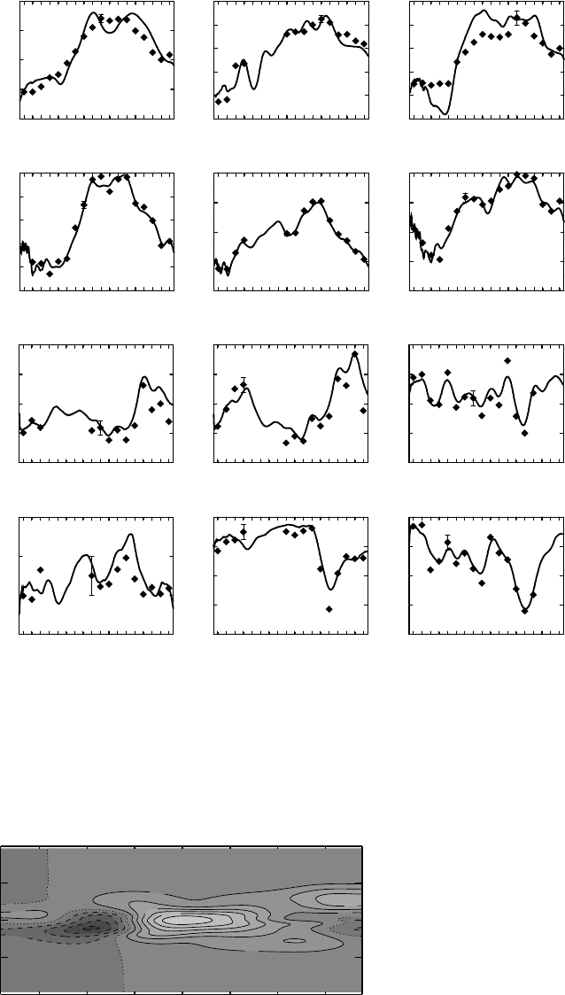
of Year 2; the best occur during the major El Ni˜no event of Year 3: see Fig. 5.5.2. The

inverse circulation ﬁelds are discussed in detail in BI and BII; only the residuals and

diagnostics will be reviewed here.

Consider for example the dynamical residual r

for the SST equation, shown in

Fig. 5.5.3 for September 30, 1994. The quantity plotted is the equivalent surface heat

ﬂux ρ

, where ρ

is the density of sea water, C

its heat capacity, and H

the thickness of the ocean surface layer. The contour interval is 20 W m

−2

. The prior

estimate of 50 W m

−2

is very signiﬁcantly exceeded over large regions, mostly on the

equator. The zonal scale of 30

◦

is that of the corresponding covariance. This ﬁeld of

residuals is one day’s distribution of heat sources and sinks that must be admitted in

the model if the local rate of change of SST is to be consistent with the TAO data.

There are two candidates for r

: the unresolved advective heat ﬂuxes (both horizontal

and vertical), and the missing heat exchange between the model ocean and the model

atmosphere. The atmospheric component of the coupled model exchanges heat with the

oceanic component at the rate

, but not vice versa. Radiative feedback from clouds

is thereby excluded. The atmospheric budget for geopotential anomaly φ is of the

form

∂φ

∂t

···=−

=−KT, (5.5.1)

where T is the SST anomaly and K is a positive constant. Thus a positive SST anomaly

(and therefore atmospheric heating) leads to a decrease in geopotential anomaly. The

region of signiﬁcant and positive r

on Sept. 30, 1994 coincides with a positive anomaly

T (see BI, Fig. 5). Hence both the model ocean and atmosphere gain heat locally on

that day. It must be concluded that r

represents mostly an unresolved convergence

DJFMAMJJASONDJFMAM

-20

DJFMAMJJASONDJFMAM

-2

DJFMAMJJASONDJFMAM

-50

100

150

DJFMAMJJASONDJFMAM

-4

-2

D J FMAMJ J ASOND J FMAM

-40

-20

D J FMAMJ J ASOND J FMAM

-1

SST

Z20

(a)

(b)

DJFMAMJJASONDJFMAM

-1

DJFMAMJJASONDJFMAM

-4

-2

DJFMAMJJASONDJFMAM

-6

-4

-2

DJFMAMJJASONDJFMAM

-4

-2

DJFMAMJJASONDJFMAM

-6

-4

-2

DJFMAMJJASONDJFMAM

-4

-2

(c)

(d)

Figure 5.5.2 Time series of the inverse estimate of the anomalous state at three TAO

moorings (5

◦

S, 0

◦

, 5

◦

N) along 95

◦

W. The centered symbols are the 30-day average

TAO data. All data of the same type are assigned the same standard error so only one

bar is shown per panel, but note that the amplitude scale and bar length vary from

panel to panel. Results here are for “Year 3” (December 1996–May 1998): (a) SST,

±0.3 K; (b) Z20, ±3 m; (c) u

, ±0.5ms

−1

; (d) v

, ±0.5 m s

−1

(after Bennett et al.,

2000).

-60

-20

100

140

E 160

E 180 160

W 140

W 120

W 100

Figure 5.5.3 Scaled

residual for the temperature

equation for day 180, Year 1

(September 30, 1994).

Contour interval: 20 W m

−2

(after Bennett et al., 2000).

160 5. The ocean and the atmosphere

of oceanic heat ﬂux, rather than a neglected exchange with the atmosphere. On

“Feb. 30” 1995, the region of signiﬁcantly negative r

(see BI, Fig. 12) coincides with

a negative anomaly T , yielding the same conclusion. On Nov. 30, 1994 negative r

coincides with positive T , possibly representing a loss from the ocean to the atmos-

phere rather than an oceanic heat ﬂux divergence. No clear evidence of loss from the

atmosphere to the ocean is seen in Year 1. In principle, both candidates for r

should be

accepted. However, scale analysis shows that an oceanic temperature source of strength

/gH)ρ

KT(ρ

)

−1

, c

being the atmospheric phase speed, g being gravity and

the air density, is an order of magnitude smaller than the prior standard deviation for

the residual r

. Thus, only oceanic heat ﬂux convergence is a credible candidate for r

The convergence may be vertical or horizontal. The model’s simple parameterization of

heat ﬂux using a simple mixing function is almost certainly signiﬁcantly in error. The

linear momentum equations in the model ocean and atmosphere do not support eddies

or instabilities such as tropical instability waves that could produce horizontal eddy

heat ﬂuxes. It should, however, be pointed out that such waves tend to be weakest during

El Ni˜no events (and 1994–1995 is no exception), and that they tend to be strongest

east of 150

◦

W. Yet Fig. 5.5.3 shows that the maximum SST dynamical residuals r

are

near 160

◦

W. Nevertheless, the oceanic momentum equations should include horizontal

advection, in addition to well-resolved vertical advection and better-parameterized

vertical mixing.

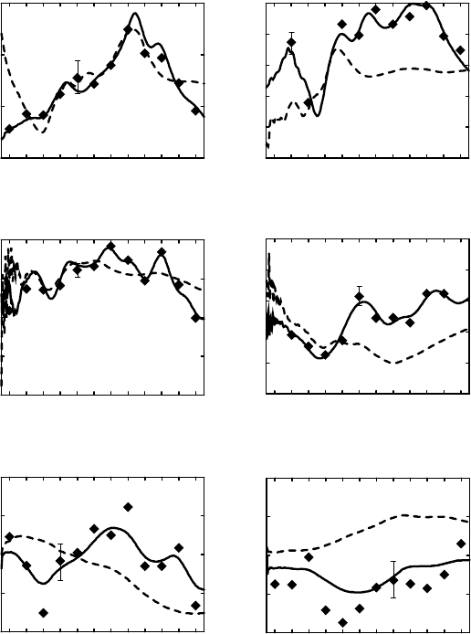
It is simple to recompute the inverse with the dynamics imposed as strong constraints:

the dynamical error variances are set to zero and the iterated indirect representer algor-

ithm is rerun. There are sufﬁciently many degrees of freedom in the initial residuals to

enable the inverse to ﬁt the data at some moorings for three months, but nowhere for

longer times: see Fig. 5.5.4 (Year 1).

Monte Carlo methods may be used to approximate the posterior error covariances:

see §3.2. These are relatively smooth and need not be computed on as ﬁne a grid as is

used for the inverse itself. A small number of samples should be adequate for such low

moments of error, if not for Monte Carlo approximation of the inverse itself. Recall that

the representers are themselves covariances (see §2.2.3), and so may be approximated

by Monte Carlo methods. Comparisons with representers and inverses calculated with

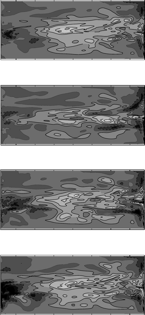
the Euler–Lagrange equations demonstrate the accuracy of sampling methods. Shown

in Fig. 5.5.5 are four calculations of SST for Nov. 1994. Daily values are calculated

as described below, and then averaged for 30 days. The ﬁrst panel shows the solution

of the Euler–Lagrange equations. This is a true ensemble estimate since it is a solution

to what are, in effect, the moment equations for the randomly forced coupled model.

The second, third and fourth panels are Monte Carlo estimates based on respectively

100, 500 and 1500 samples. It is disturbing that the +2

◦

warm pool on the Dateline,

characterizing the moderate El Ni˜no of Year 1, is only clearly expressed with 1500

samples. These calculations, variational and Monte Carlo, are all made on the same

spatial grid and at the same temporal resolution.

5.5 ENSO: testing intermediate coupled models 161

AMJ J ASONDJ FM

-1.0

0.0

1.0

2.0

SST (0

, 155

AMJ J ASONDJ FM

-3.0

-2.0

-1.0

0.0

1.0

2.0

SST (2

N, 95

AMJ J ASONDJ FM

-10.0

0.0

10.0

20.0

30.0

40.0

Z20 (8

S, 155

AMJ J ASONDJ FM

-3.0

-2.0

-1.0

0.0

1.0

S, 155

AMJ J ASONDJ FM

-1.0

0.0

1.0

2.0

3.0

S, 155

AMJ J ASONDJ FM

-60.0

-40.0

-20.0

0.0

20.0

Z20 (0

, 155

Figure 5.5.4 TAO 30-day averaged data (centered symbols) and time series

of SST, Z20, u

and v

at selected moorings. Solid lines: weak constraint

inversion; dashed lines: strong constraint inversion (Year 1, after Bennett

et al., 1998).

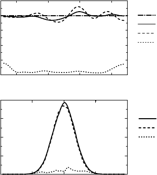
Monte Carlo approximation of the error covariances indicates a more relaxed state of

affairs. Shown in Fig. 5.5.6 are the prior and posterior variances of initial SST errors as

functions of longitude and latitude. The great difference between the prior and posterior

(or “explained”) variances, with 140 samples, greatly exceeds the sampling error in

the prior variance. The small posterior variance implies that the initial SST estimate is

reliable. Similar implications hold for the inverse estimates of SST throughout Year 1:

see BI, Figs. 17 and 18 for prior and posterior variances for that variable and other

coupled model variables. There is, however, a caveat. All these priors and posteriors

0.0

1.0

2.0

140

E 160

E 180 160

W 140

W 120

W 100

-1.0

0.0

1.0

2.0

140

E 160

E 180 160

W 140

W 120

W 100

(a)

(b)

0.0

1.0

2.0

140

E 160

E 180 160

W 140

W 120

W 100

-1.0

0.0

1.0

2.0

140

E 160

E 180 160

W 140

W 120

W 100

(c)

(d)

Figure 5.5.5 Inverse estimate of daily SST averaged for month 8, Year 1

(Nov. 1994); (a) as a solution of the Euler–Lagrange equations, (b) as a

statistical simulation with 100 samples, (c) 500 samples, (d) 1500 samples.

5.5 ENSO: testing intermediate coupled models 163

140E 180 140W 100W

)

(a)

Prior (Hyp.)

Prior (2025)

Prior (140)

Posterior (140)

30S 15S 0 15N 30N

)

(b)

Prior (2025)

Prior (140)

Posterior (140)

Figure 5.5.6 Statistical

simulations of (a) equatorial

and (b) meridional proﬁles

of prior and posterior error

variances for initial SST.

The level broken line in (a)

is the hypothesized initial

equatorial error variance of

. In (b), the hypothesis

is indistinguishable from

the solid line. The numbers

in parentheses indicate the

number of samples (after

Bennett et al., 1998).

are based on the null hypothesis for the prior errors in the initial conditions, data and

dynamics. Thus the posteriors derived from the hypothesized priors cannot be trusted

until the null hypothesis has survived signiﬁcance tests.

The prior and posterior values of the penalty functional are test statistics for the null

hypothesis: see §2.3.3. Their values for the three El Ni˜no–La Ni˜na episodes are shown

in Table 5.5.1, which is taken from BII. They are calculated using, where needed, a

Monte Carlo estimate of the full representer matrix R. Note that the prior J

and

posterior

J need only the prior data misﬁt vector h, the speciﬁed measurement error

covariance matrix C



, and the representer coefﬁcient vector

β which may be obtained

without explicit construction of R: see §3.1.4. With the exception of

J , the expectations

and variances of these statistics all do depend explicitly upon R. That the actual values

of J

in all three “Years” are signiﬁcantly less than their expected values, suggests

that the forward model is far more accurate than hypothesized. Inversion would seem

unnecessary. Yet, the actual values of

J for the three years exceed their expected

values by 15, 16 and 49 standard deviations, respectively. On the other hand, rescaling

the standard deviations of the errors in the null hypothesis by 1.40, 1.44 and 2.08,

respectively, would yield values of

J equal in each case to the expected value M

given by the number of data. Such rescalings could hardly be contested, in light of

the uncertainties involved in developing the null hypothesis. A fourth year of data, for

another El Ni˜no event, is needed in order to obtain at least one independent test of the

last upward rescaling. It would serve little purpose, as the dynamical residuals already

dominate the term balances: see Fig. 5.5.7. A rescaling of the priors might well yield a

statistically self-consistent analysis of TAO data using an intermediate coupled model,

but the model constraint would be so “slack” that it would provide no dynamical insight

into ENSO. Fully stratiﬁed models are needed, with ﬁne vertical resolution and good

estimates of moments of errors in the turbulence parameterizations.

The calculations described above involve about 4 × 10

control variables or residu-

als; there are about 2500 monthly-mean data in the 12-month episodes (Years 1 and 2)

164 5. The ocean and the atmosphere

Table 5.5.1 (a) Expected and actual values of components of the reduced penalty

functional for the intermediate coupled model (those values in parentheses are

numbers of data rather than expected values of data penalties); (b) standard

deviations (after Bennett et al., 2000).

(a) Expected and actual values

Year 1 Year 2 Year 3

M = 2624,

√

2M = 72 M = 2644,

√

2M = 73 M = 4008,

√

2M = 89

Expected Actual Expected Actual Expected Actual

16 0000 35 708 15 6000 32 028 246 132 132 140

mod

1015 1614 1022 1650 1458 3680

SST

(689) 419 (700) 717 (1088) 995

(624) 453 (628) 383 (931) 1546

(624) 396 (628) 380 (931) 940

Z20

(687) 820 (680) 678 (1058) 1129

data

1609 2088 1622 2160 2550 4614

J 2624 3702 2644 3810 4008 8322

(b) Standard deviations

Year 1 Year 2 Year 3

136 000 131 000 146 057

mod

38 38 72

data

60 59 45

J 72 73 89

DJFMAMJ JASONDJFMAM

-40

-20

(b)

(2)

)

εθ

(2)

-σ

+σ

DJFMAMJ JASONDJFMAM

-200

-100

100

200

(a)

(1)

(T+T)

(1)

-σ

+σ

Figure 5.5.7 Time series of

Year 3 term balances for the

intermediate coupled model

for (a) the anomalous SST

equation in W m

−2

(135.85

◦

W, 3.5

◦

S) and

(b) for the anomalous

lower-layer thickness

equation in 10

−6

−1

(156.38

◦

W, 0.5

◦

S). All are

daily values, spaced thirty

days apart and joined by

line segments for clarity.

The standard error σ in

(a) is 54 W m

−2

; in (b) it is

8 ×10

−6

−1

(after

Bennett et al., 2000).

5.6 Sampler of oceanic and atmospheric data assimilation 165

0 90 180 270 360

day

-5

-1

0 90 180 270 360

day

-1

SST

0 90 180 270 360

day

-4

-2

-1

0 90 180 270 360

day

-40

-30

-20

-10

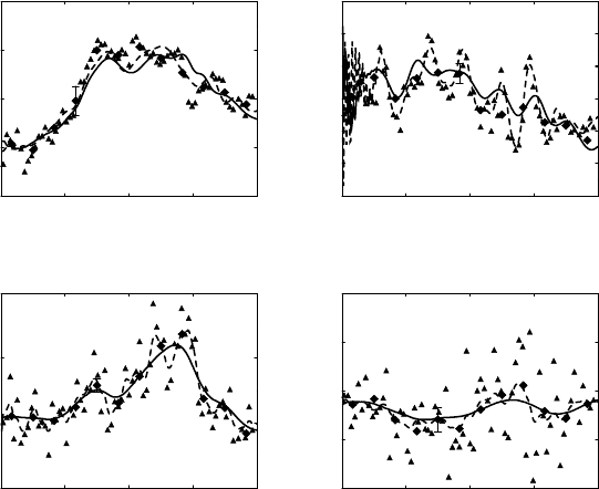
Figure 5.5.8 Time series of SST, Z20 and u

at (180

◦

) for Year 1. Diamonds:

30-day averaged data; solid lines: corresponding inverse estimate; triangles: ﬁve-day

averaged data; broken lines: corresponding inverse estimate.

and 4000 in the 18-month episode (“Year” 3). The inversion for Year 1 has been re-

peated, using ﬁve-day averaged data in place of 30-day averages. There are accordingly

about 15 000 of the former. A time series of the inverse SST is shown in Fig. 5.5.8. The

inverse is unable to ﬁt the data to within the 0.3

◦

standard error of measurement, not

because the data are of lower quality but because the time scales of the null hypothesis

and intermediate-model dynamics are too long. The ﬁgure emphasizes that the inverse

is indeed a “ﬁxed interval smoother”, and that the number M of data is not a serious

restriction on the indirect representer method. Contemporary matrix manipulation tech-

niques are not severely strained at M = 10

(see e.g., Egbert, 1997, §2.3; Daley and

Barker, 2000).

5.6

Sampler of oceanic and atmospheric

data assimilation

5.6.1 3DVAR for NWP and ocean climate models

Operational Numerical Weather Prediction relies upon timely, robust and accurate esti-

mates of initial conditions. For example, the US Navy’s Fleet Numerical Meteorology

166 5. The ocean and the atmosphere

and Oceanography Center (www.fnmoc.navy.mil) produces a global six-day fore-

cast every 12 hours using the global spectral model NOGAPS (Hogan and Rosmond,

1991), and many regional three-day forecasts every 12 hours using the regional ﬁnite-

difference model COAMPS (Hodur, 1997). The initial ﬁelds or “analyses” are created

by interpolating vast quantities of atmospheric data collected by the US Navy, and

also by civilian meteorological agencies around the world. An elementary introduction

to “Optimal Interpolation” may be found in §2.2.4. The operational “OI” scheme at

FNMOC involves multiple random ﬁelds; the priors or ﬁrst guesses or “backgrounds”

for these ﬁelds are previous predictions for that time, while data are admitted through

a time window of minus and plus three hours (implying that the analysis time is at least

three hours in the past). For comprehensive details of FNMOC’s MultiVariate Optimal

Interpolation analysis (“MVOI”), see Goerss and Phoebus (1993). Most importantly, the

prior covariances for the velocity and geopotential ﬁelds assume geostrophy (5.1.39).

However, the resulting analysis is nongeostrophic since the background ﬁeld is a pre-

diction made by a Primitive Equation model.

The essential computational task in an OI scheme is solving the linear system

+ C



}β = d − u

(5.6.1)

for the coefﬁcients β of the covariances C

(x, t) in (2.2.22). Recall that d is the vector

of data, while u

is the vector of “measured” values of the background u

(x, t). Note

that MVOI replaces the single spatial coordinate x in (2.2.22) with three spatial co-

ordinates, one of which may be pressure as in (5.1.1). The dimension of the system is the

number of data, which can be in excess of 10

in a global analysis. MVOI reduces the di-

mension by analyzing the data in regions. The coefﬁcient matrix in (5.6.1) is symmetric

and positive deﬁnite, so MVOI solves the system by Cholesky factorization (Press et al.,

1986, §2.9). Should small negative eigenvalues be encountered, MVOI arbitrarily

increases the diagonal of C



, that is, it increases the variances of the measurement

errors until positivity is restored.

The solution of (5.6.1) also mimizes the penalty function

J [β] =

+ C



}β − β

(d − u

). (5.6.2)

Preconditioned conjugate gradient searches (Press et al., 1986, §10.6) for the unique

minimum of J may be efﬁciently implemented on multiprocessor computers. System

dimensions of 10

or larger can be managed, and so regionalization is not necessary.

This algorithm for implementing OI has become known as “3DVAR”, and is being

introduced at many NWP centers such as FNMOC (Daley and Baker, 2000), at the

United Kingdom Meteorological Ofﬁce (Lorenc et al., 2000) and at the NASA Global

Modeling and Assimilation Ofﬁce (www.polar.gsfc.nasa.gov). Oceanographers

can learn much from these operational NWP centers, concerning the real-time quality-

control of vast data sets and the devising of prior multivariate covariances.

A fast algorithm for the spatial “convolution” (3.1.25), essential to efﬁcient im-

plementation of physically realizable inverse models, is also required for 3DVAR.