Bennett A.F. Inverse Modeling of the Ocean and Atmosphere

4.2 Sweep algorithm 97

The system (4.2.15), (4.2.17), (4.2.21) and the system (4.2.16), (4.2.18), (4.2.22) may

be integrated forward in time until t = t

−. Note that the initial value and forcing

for P(x, y, t), respectively C

(x, y) and Q

(x, y), are symmetric. If we assume that

P(x, y, t) is symmetric, then by (4.2.21)

P(x, 0, t) = P(0, x, t) = cQ

δ(x), (4.2.23)

and hence the seemingly symmetry-breaking fourth term on the lhs of (4.2.15) is

cP(x, 0, t)δ(y) = c

δ(x)δ(y), (4.2.24)

which is symmetric. In other words, assuming symmetry leads to no contradiction.

It remains to determine the jumps in P and v as t passes through t

. First, we learn

from (4.2.12) that λ is discontinuous in t

, with

−λ(x, t

+) + λ(x, t

−) = (d

−

)







−1

δ, (4.2.25)

where (δ)

= δ(x − x

). We infer from (4.2.4) that

u is continuous at t

. Hence (4.2.9)

implies that







dyP(x, y, t )λ(y, t ) + v(x, t)





−

= 0 . (4.2.26)

Substitute (4.2.14) into (4.2.25) and then substitute (4.2.25) into (4.2.26). Equating

terms proportional to λ(x, y, t

−) yields, after a little algebra,

P(x, y, t

+) − P(x, y, t

−)

=−P

k−

(x)



k−

+ C





−1

k−

(y) (4.2.27)

and

v(x, t

+) − v(x , t

−) = K

− v

k−

), (4.2.28)

where

k−

(x) ≡ P(x

, x, t

−) (4.2.29)

k−

≡ P(x

, x

, t

−) (4.2.30)

≡







−1

(4.2.31)

and

k−

)

= v(x

, t

−). (4.2.32)

We now have an explicit algorithm for P and v, for all t ≥ 0. To complete the formula

(4.2.9) for

u, we need λ.Nowλ obeys (4.2.1)–(4.2.3), but (4.2.1) involves

u.Wemay

eliminate

u using (4.2.14), yielding an equation for P, v and λ. We can determine P

and v,soλ may be found by backwards integration, and the Gelfand and Fomin sweep

is complete.

98 4. The varieties of linear and nonlinear estimation

Exercise 4.2.2

Derive the equation for λ, free of

u. 

Note 1. The above procedure has a major drawback: it would be necessary to

compute and store P(x, y, t) and v(x, t) for 0 < x, y < L, and for 0 < t < T .

This would be prohibitive in practice.

Note 2. It is only necessary to store P(x, y, t

+) and v(x, t

+) in order to evaluate

, for 1 ≤ k ≤ K , and hence λ (see(4.2.12)). Having solved for λ, we could

then ﬁnd

u by integrating (4.2.4)–(4.2.6).

Note 3. There are other such “control theory” algorithms such as that of Rauch, Tung

and Streibel (e.g., Gelb, 1974), but these require even more computation and

storage. These algorithms are impractical for the generalized inversion of

oceanic or atmospheric models.

Note 4. The adjoint variable λ vanishes after assimilating the last data: λ = 0 for

< t < T , hence the generalized inverse

u agrees with the “intercept” v at

the end of the smoothing interval:

u(x, t) = v(x, t) (4.2.33)

for t

< t < T , where T is somewhat arbitrary. So, if we only want to know

the inﬂuence of the K

(the latest) data d

upon the circulation estimate

u at

time t

(the present), then we need not do more than solve for v (which requires

solving for P: see (4.2.28)–(4.2.32)). The previous data: d

,...,d

K −1

also

inﬂuence v at time t

,butd

has no inﬂuence on v for t < t

. Thus v is a

“sequential” estimate of u, using data as they arrive.

4.3

The Kalman ﬁlter: statistical theory

4.3.1 Linear regression

The Kalman ﬁlter has just been derived as a ﬁrst step in solving linear Euler–Lagrange

problems. It is a sequential algorithm, that is, it calculates the generalized inverse at

times later than all the data: v(x, t) =

u(x, t) for all t > t

. Recall that

u minimizes a

quadratic penalty functional over 0 ≤ t ≤ T , where t

< T . The Kalman ﬁlter will now

be derived using linear regression.

4.3.2

Random errors: ﬁrst and second moments

Our ocean model is

∂u

∂t

+ c

∂u

∂x

= F + f, (4.3.1)

4.3 The Kalman ﬁlter: statistical theory 99

for 0 ≤ x ≤ L and 0 ≤ t ≤ T , subject to the boundary condition

u(0, t ) = B(t) +b(t) (4.3.2)

and the initial condition

u(x, 0) = I (x) + i (x). (4.3.3)

We have assumed that F, B and I are unbiased estimates of the forcing, boundary and

initial values:

Ef = Eb = Ei = 0, (4.3.4)

and we prescribed the autocovariances of f , b and i :

E( f (x, t) f (y, s)) = Q

(x, y)δ(t − s), (4.3.5)

E(b(t)b(s)) = Q

δ(t − s), (4.3.6)

E(i(x)i(y)) = C

(x, y). (4.3.7)

We assumed that their cross-covariances all vanish: E( fb) = E( fi) = E (bi) = 0.

There are data at N points x

,...,x

, at discrete times t = t

,...,t

= u(x

, t

) + 

(4.3.8)

for 1 ≤ n ≤ N , where 

are the measurement errors, for which

E

= E( f 

) = E(b

) = E(i

) = 0, (4.3.9)

E(



) = δ



. (4.3.10)

That is, f , b and 

are uncorrelated in time. The vectors in (4.3.9), (4.3.10) have

N components. Note that the points x

,...,x

do not necessarily coincide with a

spatial grid for numerical integration of (4.3.1)–(4.3.3); they are merely a set of N

measurement sites.

4.3.3

Best linear unbiased estimate: before data arrive

We shall now construct w(x, t), the best linear unbiased estimate of u(x, t), given data

prior to t. Assuming t

> 0, at time t = 0 we can do no better than

w(x, 0) = I (x), (4.3.11)

for which the error variance is C

: see (4.3.7). For 0 ≤ t ≤ t

−, let

∂w

∂t

+ c

∂w

∂x

= F, (4.3.12)

w(0, t) = B(t). (4.3.13)

100 4. The varieties of linear and nonlinear estimation

The error e ≡ u − w obeys

∂e

∂t

(x, t) +c

∂e

∂x

(x, t) = f (x, t), (4.3.14)

e(x, 0) = i(x), (4.3.15)

e(0, t ) = b(t), (4.3.16)

the solution of which is

e(x, t) =



ds dξγ(ξ,s, x, t) f (ξ,s) + c



ds γ (0, s, x, t)b(s)



dξγ(ξ,0, x, t)i (ξ ), (4.3.17)

where γ is the Green’s function (see §1.1.4). Hence E (e(x, t) f (y, t)) =

(x, y),

since γ (x, t, y, t) = δ(x − y), and

t−

δ(s) ds =

. Also

E(e(x, t)b(t)) = cQ

δ(x). (4.3.18)

Now deﬁne the spatial error covariance at time t by

P(x, y, t) ≡ E(e(x , t)e(y, t)) = P(y, x, t). (4.3.19)

Multiplying (4.3.14) by e(y, t) and averaging yields

∂P

∂t

(x, y, t) + c

∂P

∂x

(x, y, t) + c

∂P

∂y

(x, y, t) = Q

(x, y); (4.3.20)

multiplying (4.3.16) by e(y, t) and averaging yields

P(0, y, t) = cQ

δ(y), (4.3.21)

P(x, 0, t) = cQ

δ(x). (4.3.22)

Initially,

P(x, y, 0) = C

(x, y). (4.3.23)

4.3.4

Best linear unbiased estimate: after data have arrived

The situation at time t

− is that we have an estimate w

−

(x) ≡ w(x, t

−), equal to the

mean of u(x, t

), and we have its error covariance P

−

(x, y) ≡ P(x, y, t

−). The new

information are the data d

. These too contain random errors, but by (4.3.8) we are

assuming that

= Eu

. (4.3.24)

Let us seek a new estimate w

(x) for u(x, t

) which is linear in w

−

(x) and associated

data misﬁts:

(x) = αw

−

(x) + s(x)

− w

−

), (4.3.25)

4.3 The Kalman ﬁlter: statistical theory 101

where

−

)

= w

−

) ≡ w(x

, t

−). (4.3.26)

The constant α and the interpolant s(x) have yet to be chosen. Consider the error

(x) = u(x, t

) − w

(x). (4.3.27)

Now

u(x, t

) = w

−

(x) + e

−

(x), (4.3.28)

where e

−

(x) = e(x , t

−). Hence

(x) = (1 − α)w

−

(x) + e

−

(x) − s(x)

− w

−

). (4.3.29)

But Ee

−

= 0. So if we choose α = 1, then

(x) = 0 (4.3.30)

and (4.3.25) is an unbiased estimate. The error variance is

(x, x) = E



(x)



. (4.3.31)

Exercise 4.3.1

Show that the error variance (4.3.31) is least if the optimal interpolant is

s(x) = K

(x), (4.3.32)

where the “Kalman gain” vector ﬁeld K

(x) in (4.3.32) is

(x) =

−

+ C



(

−1

−

(x). (4.3.33)

The vector P

−

(x) and matrix P

−

have components

n−

(x) = P

−

, x),

nm−

= P

−

, x

). (4.3.34)



Exercise 4.3.2

Show that the posterior error covariance at time t

(x, y) ≡ E



(x)e

(y)



= P

−

(x, y) − P

−

(x)

−

+ C



(

−1

−

(y). (4.3.35)



Clearly, we may repeat this construction at t

, t

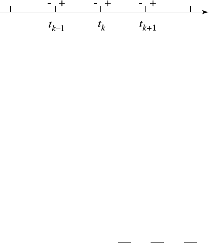
,.... See Fig. 4.3.1.

Gathering up all the results, the Kalman ﬁlter estimate w satisﬁes

∂w

∂t

+ c

∂w

∂x

= F (4.3.36)

102 4. The varieties of linear and nonlinear estimation

Figure 4.3.1 Time line for

the Kalman ﬁlter.

for 0 ≤ x ≤ L, t

< t < t

k+1

, subject to

w(x, 0) = I (x) (4.3.37)

and

w(0, t) = B(t). (4.3.38)

The change in w at time t

w(x, t

+) − w(x, t

−) = K

(x)

− w

−

), (4.3.39)

where the Kalman gain is

(x) =

−

+ C



(

−1

−

(x). (4.3.40)

The error covariance satisﬁes

∂ P

∂t

+ c

∂ P

∂x

+ c

∂ P

∂y

= Q

(4.3.41)

for 0 ≤ x, y ≤ L, t

< t < t

k+1

, subject to

P(0, y, t) = cQ

δ(y), (4.3.42)

P(x, 0, t) = cQ

δ(x) (4.3.43)

and

P(x, y, 0) = C

(x, y). (4.3.44)

The change in P at t

P(x, y, t

+) − P(x, y, t

−) =−P

−

(x)

(y). (4.3.45)

The new data always reduce the error variance at data sites. Note carefully the assump-

tions that the dynamical and boundary errors f , b and the data 

are uncorrelated in

time, and that the different types of errors are not cross-correlated. Note also that the

optimal choices for α and s(x) in (4.3.25) are not random. They depend not upon the

random inputs w

−

(x), d

but upon the covariances of the errors in the inputs.

4.3.5

Strange asymptotics

It is usually assumed that the data errors are statistically stationary, that is, C



is indepen-

dent of k. It is often the case that the temporal sampling interval t

k+1

− t

also is indepen-

dent of k. Consequently, the Kalman ﬁlter error covariance P approaches an equilibrium

state, in which P(x, y, t

−) = P(x, y, t

k+1

−) and P(x, y, t

+) = P(x, y, t

k+1

+). The

4.3 The Kalman ﬁlter: statistical theory 103

covariance does still evolve in time from t

+ to t

k+1

−,butQ

and Q

are independent

of t and so the evolution is the same in every data interval. In general we are interested

in more complicated dynamics than are expressed in (4.3.1); so long as the dynamics

are linear, they may be expressed as

∂u

∂t

+ L

u = F + f, (4.3.46)

where L

is a linear partial differential operator with respect to x. Of course, Primitive

Equation models involve many dependent variables, but we shall retain just one here,

namely u, for clarity. The error covariance now satisﬁes

∂ P

∂t

(x, y, t) + L

P(x, y, t) + L

P(x, y, t) = Q

(x, y). (4.3.47)

To simplify the discussion further, let us assume that the data interval t = t

k+1

− t

is much smaller than the evolution time scale for (4.3.47), so that (see Fig. 4.3.1)

−

= P

− t(L

−

+ L

−

) + tQ

+ O(t

), (4.3.48)

where P

−

= P(x, y, t

k+1

−) and P

= P(x, y, t

+). Recall that both P

and P

−

are

independent of k at equilibrium, hence (4.3.40) and (4.3.45) yield

= P

−

− P

−

+ C



)

−1

−

. (4.3.49)

Combining (4.3.48) and (4.3.49) we have

t(L

−

+ L

−

) + P

−

+ C



)

−1

−

= tQ

+ O(t

). (4.3.50)

Notice the nonlinearity of the impact of data sites upon P. It is possible for P to strike

a balance between the two terms on the left-hand side of (4.3.50) (dynamics and data-

impact). This balance can take the form of a boundary layer around data sites. The

Kalman gain K and the Kalman ﬁlter estimate w will have this structure, which is quite

unphysical (Bennett, 1992). It arises from the adoption of a “cycling” algorithm, as in

(4.3.45).

Exercise 4.3.3

Show that there is no such nonlinearity in the non-sequential representer algorithm,

for one ﬁxed smoothing interval [0, T ] that may include many measurement times:

0 < t

< ···< t

< T . 

Exercise 4.3.4

Consider smoothing a sequence of such intervals: KT < t < (K + 1)T , K = 0, 1,

2,..., using the inverse estimate at the end of the K

interval as the ﬁrst-guess initial

ﬁeld at the start of the (K + 1)

: I

K +1

(x) =

(x, (K + 1)T ), and using the error

covariance for the inverse estimate as the error covariance for the ﬁrst-guess initial

ﬁeld: C

K +1

(x, y) = C

(x, y, (K + 1)T ). Show that the equilibrium error covariance

for this “cycling” inverse obeys a nonlinear equation like (4.3.50). Hint: for simplicity,

104 4. The varieties of linear and nonlinear estimation

assume that the domain is inﬁnite: −∞ < x < ∞, assume that the ﬁrst-guess forcing

ﬁeld F

is perfect: C

= 0, and integrate (3.2.43) as crudely as (4.3.48). 

4.3.6

“Colored noise”: the augmented Kalman ﬁlter

We may relax the assumption (4.3.5) of “white system noise”. The simplest “colored

system noise” has covariance

E( f (x, t) f (y, s)) = Q

(x, y)e

−

|t−s|

(4.3.51)

for some decorrelation time scale τ>0. Note that the Q

s appearing in (4.3.5) and

(4.3.51) have different units of measurement. It may be shown that (4.3.51) is satisﬁed

by solutions of the ordinary differential equation

(x, t) −τ

−1

f (x, t) = q(x, t), (4.3.52)

provided

E(q(x, t)q(y, s)) = (τ/2)

−1

(x, y)δ(t − s), (4.3.53)

E( f (x, 0) f (y, 0)) = Q

(x, y), (4.3.54)

and

E( f (x, 0)q(y, s)) = 0. (4.3.55)

This suggests augmenting the state variable (Gelb, 1974):

u(x, t) →



u(x, t)

f (x, t)



. (4.3.56)

The dynamical model is now (4.3.46), (4.3.52). Note that the “colored” random process

f (x, t) is now part of the state to be estimated. The augmented system is driven by the

“white noise” q(x, t). The augmented error covariance now includes cross-covariances

of errors in the Kalman ﬁlter estimates of u and f .

4.3.7

Economies

The Kalman ﬁlter is a very popular data assimilation technique, owing to its being se-

quential (e.g., Fukumori and Malanotte-Rizzoli, 1995; Fu and Fukumori, 1996; Chan

et al., 1996). Also, the “analysis” step (4.3.39) is identical to synoptic or spatial optimal

interpolation, as widely practiced already in meteorology and oceanography (Miller,

1996; Malanotte-Rizzoli et al., 1996; Hoang et al., 1997a; Cohn, 1997). The Kalman

ﬁlter algorithm evolves the error covariance P in time, via (4.3.41), and (4.3.45).

Nevertheless, evolving P is a massive task for realistically large systems so many

compromises are made. For example, the covariance P(x, y, t ) is evolved on a compu-

tational grid much coarser than the one used for the state estimate w(x , t), or P(x, y, t)

4.4 Maximum likelihood 105

is integrated to an equilibrium covariance P

∞

(x, y) which is then used at all times

,...,t

(Fukumori and Malanotte-Rizzoli, 1995), or the number of degrees of free-

dom in w(x , t) is reduced by an expansion in spatial modes (Hoang et al., 1997b). A

covariance such as P may also be approximated by statistical simulation, as discussed

in §3.2.

4.4

Maximum likelihood, Bayesian estimation,

importance sampling and simulated annealing

4.4.1 NonGaussian variability

Least-squares is the simplest of all estimators. It has so many merits. Gradients and

Euler–Lagrange equations are available, so long as the dynamics are smooth. Structural

analyses in terms of null spaces, data spaces, representers and sweep algorithms are

available, as are statistical closures such as the Kalman ﬁlter, when the dynamics are

linear or linearizable. Why, then, choose other estimators? Consider ocean temperatures

near the Gulf Stream front. As the latter meanders back and forth across the mooring,

the temperature switches rapidly between the higher value for the warm Sargasso Sea

water and the lower value for the cool slope water. Thus the frequency distribution of

temperature would be bimodal, with peaks at the two values. A least-squares analysis of

temperature would yield the average temperature, which is in fact realized only brieﬂy

while the front is passing through the mooring. What would be a more suitable estima-

tor? Can samples of the non-normal population be generated? How can its estimator

be minimized?

4.4.2

Maximum likelihood

Let us review some introductory statistics. Suppose the continuous random variable

u has the probability distribution function p(u; θ), where θ is some parameter. Let

,...,u

be independent samples of u. Then the joint pdf of the samples is the

likelihood function:

L(θ) = p(u

,...,u

; θ) =

)

i=1

p(u

; θ). (4.4.1)

That is, L

i=1

is the probability that the n samples are in the respective intervals

, u

+ du

), 1 ≤ i ≤ n. The maximum likelihood estimate of θ is that value of θ for

which L(θ) assumes its maximum value.

As an illustration, suppose that u is normally distributed with mean µ and

variance σ

p(u; µ, σ ) = (2πσ

)

−

exp[−(2σ

)

−1

(u − µ)

]. (4.4.2)

106 4. The varieties of linear and nonlinear estimation

Note that there are two parameters here: µ and σ .Givenn samples of u, what are the

maximum likelihood estimates of µ and σ

? The likelihood function is

L(µ, σ ) ≡

)

i=1

p(u

; µ, σ ) (4.4.3)

= (2πσ

)

−n/2

exp

−(2σ

)

−1



i=1

− µ)

. (4.4.4)

We may as well seek the maximum of

l = log L =−

log(2πσ

) − (2σ

)

−1



i=1

− µ)

. (4.4.5)

Extremal conditions are

∂l

∂µ

=−2(2σ

)

−1



i=1

− µ) = 0, (4.4.6)

∂l

∂(σ

)

=−

−2

−4



i=1

− µ)

= 0. (4.4.7)

The ﬁrst condition yields

= n

−1



i=1

, (4.4.8)

the second yields

= n

−1



i=1

− µ

)

. (4.4.9)

So µ

, the maximum likelihood estimate for µ, is just the arithmetic mean, while σ

is just the sample variance.

Now suppose that the pdf for u is exponential, centered at µ and with scale σ :

p(u; µ, σ ) = (2σ )

−1

exp[−σ

−1

|u − µ |]. (4.4.10)

Then

L(µ, σ ) = (2σ )

−n

exp

−σ

−1



i=1

− µ|

, (4.4.11)

l(µ, σ ) =−n log(2σ ) − σ

−1



i=1

− µ|. (4.4.12)

Hence

∂l

∂µ

=−σ

−1





µ>u

1 −



µ<u



= 0, (4.4.13)

Bennett A.F. Inverse Modeling of the Ocean and Atmosphere

Подождите немного. Документ загружается.