Bemelmans J. et. al. (editor) Elliptic and Parabolic Problems: Rolduc and Gaeta 2001
Подождите немного. Документ загружается.

120
3 A simple example
We consider in this section, as an example, the one-dimensional version of the stationary
problem corresponding to problem (11)-(14), with }i{u\,u
2
) = 0, i = 1,2, and non-flux
boundary conditions, as stated in [27]. Notice that this choice of boundary conditions
and source terms implies the conservation of the number of individuals of each of the
species. This may be regarded as a simple equilibrium model of a dynamics in which
population pressure effects are much faster than growth and competition effects. For the
study of the long-time behaviour of solutions in the case in which interaction of pressure
and growth-competition terms are present (no environmental potential), the reader is
refered to [24].
We shall see that this rather simple example already exhibits the phenomena of seg-
regation of populations. We obtain necessary conditions relating transport and cross-
diffusion coefficients. Sufficient conditions either involves the size of the solution or are
just a consequence of a very steep difference between the transport coefficients of both
equations.
Integrating the equations that one obtains when dropping the time derivative and the
source terms of equations (11) in (0,:r), with ie(l, and using the boundary conditions,
we obtain the following problem. Find {ui,u
2
) : O x Q
—>•
R^_ such that
(«i(ci + a
1
u
1
+ u
2
))' + dxqui =0 .
[U
2
(c
2
+
<l2«2
+ Ml)) +
d
2
qU2
= 0
with
/ ui = u\ and / u
2
~ u
2
. (30)
Ja in
Here, U\ and u
2
stand for the mass of u\ and u
2
, respectively. We have the following exis-
tence result, which is independent of the size of the non-negative parameters a*. Therefore,
condition (9) is not necessary in this example, too.
Proposition 1 Let c\ and c
2
be
positive and assume q e L°°(fi). There exists a solution
(ui,u
2
) of Problem (29)-(30) such thatui,u
2
> 0 in
CI
andu\,u
2
6 W
1,a
°(Q). In addition,
ifqe H""'°°(fl) then the solution (u
u
u
2
) satisfies u
u
u
2
6 W™
+1
'°°(n).
The proof is straightforward. We just rewrite equations (29)-(30) as
U, (31)
gfei(Mi,M
2
)
ni
, _ _qh
2
{ui,u
2
)
u,
g{ui,u
2
) ' g(u
u
u
2
)
with
g(ui, u
2
) := (ci + 2a
1
u
1
+ u
2
)(c
2
+ 2a
2
u
2
+ ui) - uiu
2
> 0,
hi(ui,u
2
) := di(c
2
+ 2a
2
u
2
+ ui) - d
2
u
2
, (32)
h
2
{ux,u
2
) := d
2
(ci + 2ai«i + u
2
)
—
diU^.
Then, we use an iterative scheme on the representation formulae of the solutions given by
i \ m\
f
[
x
-qhi(u
lt
u
2
)
x
[ f
x
-qh
2
{ui,u
2
),
Ui{x) = «i(0) exp{ / ——
;
r-}, u
2
{x) = w
2
(0) exp{ / ^ r^}, (33)
JO »l(«l>«2) Jo MMl.Ua)
121
with ui(0),u
2
(0) determined by (30) (see [10] for details).
We now discuss the notion of segregation in a simplified framework. We shall assume,
following [27], that the environmental potential U(x) is a smooth function such that the
corresponding enviromental flux satisfies q(x
0
) = 0 for a single point x
0
€ fi.
Definition 1 We say that the stationary problem (29)-(30) has the property of segrega-
tion if there exists a point
XQ
£ Q such that u\ and u
2
have a
local
maximum and minimum
at
XQ,
respectively (or vice versa).
Observe that, since q(xo) = 0, from (31) we find u\(x
0
) = u'
2
(x
0
) = 0, so we deduce
the existence of a critical point, x
0
, both for ui and u
2
. Taking derivatives in (31) and
evaluating at
Xo
we obtain
g(u
1
(x
0
),u
2
{x
0
))u"(x
0
) = -q
J
{x
0
)h
1
(ui(xo),U2{x
0
)),
g(u
1
(x
0
),U2(x
0
))u2(x
0
) = -q'{xo)h
2
(u
1
(xo),U2(xo)).
Therefore, segregation will take place if hi(ui(x
0
),u
2
(x
0
))h
2
(ui(x
0
),u
2
{x
Q
)) < 0. ^From
(32) we see that this is equivalent to one of the following conditions:
u
2
(x
0
)(d
i
- 2o
2
di) > di(c
2
+ ui(z
0
)), ui(x
0
)(di - 2aid
2
) > rf
2
(ci + u
2
(x
0
)). (34)
In the trivial case in which d\d
2
< 0, segregation does always occur. Notice that in
this case x
0
is an attractive point (from the environmental point of view) for one of
the populations and a repulsive point for the other. We may then analyze the case
di > 0, i = 1,2 (the case di < 0 is similar). From (34) we obtain a necessary condition
involving the diffusion coefficients, namely d
t
> 2a
t
dj, i,j = 1,2, i ^ j. Observe that if
none of these conditions are satisfied (no segregation) then the coefficients oi, a
2
satisfy
a\a
2
> 1/4, which is a condition in the same spirit as (9). On the other hand, since the
L°° norms of «; are bounded when di
—>
0, i = 1,2, see [10], we conclude that a sufficient
condition for segregation is that
di/d
2
is large or small enough.
We discretized problem (11)-(14), with no-flux boundary conditions and zero source
terms,
by a semi-implicit finite difference method and let tend t
—>
oo in order to obtain
steady-state solutions. The numerical experiments conducted show that, for a wide range
of model parameters and initial conditions, the numerical scheme is stable, which allows us
to show some different behaviours of the two interacting species included in the model. In
particular, it is interesting to observe when segregation of the two species, due to habitat
hetereogenity, does appear. We also used an iterative scheme based on the formulae (33)
and could verify that the solutions of (11)-(14), obtained in the large-time limit, coincide
with the solutions of the iterative scheme.
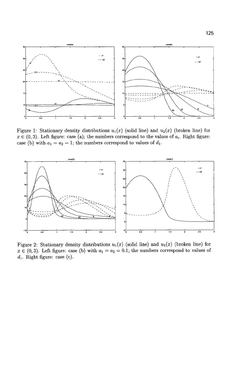
We show here numerical experiments corresponding to the following cases:
(a) Large and smallcross-diffusion terms. Set c; = d
t
= 1 and constant initial conditions
Mio = 10, «2o = 20. Then small a* correspond to large cross-diffusion and vice
versa. Figure 1 shows the numerical solution of model corresponding to values of
Oi = 0,0.1,10.
122
(b) Segregation effects
due to
different transport coefficients,
i.e. di 3> d
2
. Set c
t
= d
2
=
1
and
tiio
=
10,
u
2
o =
10. Figure
1
shows
the
numerical solutions corresponding
to
a
i
=
0,2
= 1 and d\ =
4,8,20,40.
As
case
(a)
shows, large cross-diffusion enhance
segregation effects, therefore
we
repeat
the
last simulation with
a; =
0.1. Figure
2
shows
the
same results
as
before also
for
this case.
(c)
Set
Ci
= 1, ai = 1, a
2
=
0.01,
di = 40, d
2
= 1,
Mio
=
W20
= 10
(Figure
2).
Here,
a
neat segregation
of the two
species
can be
observed.
Acknowledgements
The authors acknowledge partial support from
the TMR
Project "Asymptotic methods
in kinetic theory", grant number ERB-FMBX-CT97-0157
and
from
the
DAAD Project
"Acciones Integradas".
The
first
and
second authors were supported
by the
Spanish
Ministerio
de
Ciencia
y
Tecnologia, project number MCT-OO-BFM-1324.
The
last author
was supported
by the
Gerhard-Hess Program
of the
Deutsche Forschungsgemeinschaft,
grant
JU
359/3,
and by the AFF
Project
of
the University
of
Konstanz, grant
4/00.
References
[1]
H.
Amann
and
M. Renardy. Reaction-diffusion problems
in
electrolysis. Nonlin.
Diff.
Eqs.
Appl., 1:91-117,
1994.
[2]
N.
Boudiba
and M.
Pierre. Global existence
for
coupled reaction-diffusion equations
systems.
J.
Math. Anal. Appl, 250:1-12, 2000.
[3]
Y.
Choi
and R. Lui.
Multi-dimensional electrochemistry model. Arch.
Rat.
Mech.
Anal, 130:315-342,
1995.
[4]
P.
Degond,
S.
Genieys,
and A.
Jiingel. Symmetrization
and
entropy inequality
for
general diffusion equations.
C. R.
Acad.
Sci.
Paris, 325:963-968,
1997.
[5]
P.
Deuring.
An
initial-boundary value problem
for a
certain density-dependent
dif-
fusion system. Math.
Z.,
194:375-396,
1987.
[6]
Z.
Duan
and L.
Zhou. Global
and
blow-up solutions
for
nonlinear degenerate
parabolic systems with crosswise diffusion.
J.
Math. Anal. Appl, 224:263-278, 2000.
[7]
R.
Eisenberg
and D.
Gillespie.
A
singular perturbation
of
the Poisson-Nernst-Planck
system: application
to ion
channels. Preprint,
1999.
[8]
G.
Gagneux
and
M. Madaune-Tort. Analyse mathematique
de
modeles
non
lineaires
de I'ingenierie petroliere. Springer, Paris,
1996.
[9]
H.
Gajewski
and K.
Zacharias. Global behaviour
of a
reaction-diffusion system mod-
elling chemotaxis. Math. Nachr., 195:77-114,
1998.
123
[10]
G.
Galiano, M. Garzon, and A. Jiingel. Analysis and numerical solution of a nonlinear
cross-diffusion system arising
in
population dynamics. To appear
in
Revista de la Real
Academia
de
Ciencias Exactas,
Fis. y Nat,
2002.
[11]
G.
Galiano,
M.
Garzon,
and A.
Jiingel. Semi-discretization
in
time
and
numerical
convergence
of
solutions
of a
nonlinear cross-diffusion system arising
in
population
dynamics. Submitted
for
publication, 2000.
[12]
M. T. Gyi and A.
Jiingel.
A
quantum regularization
of
the one-dimensional hydro-
dynamic model
for
semiconductors.
Adv. Diff.
Eqs., 5:773-800, 2000.
[13]
H.
Hoshino. Nonnegative global solutions
to a
class
of
strongly coupled reaction-
diffusion systems. Advances
Diff.
Equ., 5:801-832, 2000.
[14]
T.
Ichikawa
and Y.
Yamada. Some remarks
on
global solutions
to
some quasilinear
parabolic system with cross-diffusion. Funkcialaj Ekvacioj, 43:285-301, 2000.
[15]
A.
Jiingel. Quasi-hydrodynamic Semiconductor Equations. Progress
in
Nonlinear
Differential Equations
and Its
Applications. Birkhauser, Basel, 2001.
[16]
A.
Jiingel
and
Y.-J. Peng.
A
hierarchy
of
hydrodynamic models
for
plasmas. Zero-
electron-mass limits
in
the drift-diffusion equations. Annales H. Poincare, 17:83-118,
2000.
[17]
A. S.
Kalashnikov. Some problems
of
the qualitative theory
of
non-linear degenerate
second-order parabolic equations. Russ. Math. Surveys, 42:169-222,
1987.
[18]
J.
Kamel
and M.
Kirane. Pointwise
a
priori bounds
for a
strongly coupled system
of reaction-diffusion equations with
a
balance law. Math. Meth. Appl.
Sci.,
21:1227-
1232,
1998.
[19]
J.U. Kim.
Smooth solutions
to a
quasi-linear system
of
diffusion equations
for a
certain population model. Nonlin. Anal, 8:1121-1144, 1984.
[20]
Y. Lou and
W.-M.
Ni.
Diffusion, self-diffusion
and
cross-diffusion.
J. Diff. Eqs.,
131:79-131,
1996.
[21]
Y. Lou and
W.-M.
Ni.
Diffusion,
vs.
cross-diffusion:
an
elliptic approach.
J. Diff.
Eqs.,
154:157-190,
1999.
[22]
Y.
Lou, W.-M.
Ni, and
Y. Wu.
The
global existence
of
solutions
for a
cross-diffusion
system.
Adv.
Math., Beijing, 25:283-284, 1996.
[23]
P. A.
Markowich,
C. A.
Ringhofer,
and C.
Schmeiser. Semiconductor Equations.
Springer, 1990.
[24]
M.
Mimura and K. Kawasaki. Spatial segregation
in
competitive interaction-diffusion
equations.
J.
Math. Biol., 9:49-64,
1980.
124
[25] K. Post. A non-linear parabolic system modeling chemotaxis with sensitivity func-
tions.
Preprint, Humboldt-Universitat Berlin, Germany, 1999.
[26] M. Pozio and A. Tesei. Global existence of solutions for a strongly coupled quasilinear
parabolic system. Nonlin. Anal., 14:657-689, 1990.
[27] N. Shigesada, K. Kawasaki, and E. Teramoto. Spatial segregation of interacting
species. J. Theor. Biol., 79:83-99, 1979.
[28] J. Simon. Compact sets in the space
V(0,T;
B). Ann. Math. Pura AppL, 146:65-96,
1987.
[29] Y. Wu. Qualitative studies of solutions for some cross-diffusion systems. In T.-T.
Li,
M. Mimura, Y. Nishiura, and Q.-X. Ye, editors, China-Japan Symposium on
Reaction-Diffusion Eqautions and Their Applications and Computational Aspects,
pages 177-187, Singapore, 1997. World Scientific.
[30] A. Yagi. Global solution to some quasilinear parabolic system in population dynam-
ics.
Nonlin. Anal., 21:603-630, 1993.
125
Figure 1: Stationary density distributions u\{x) (solid line) and u
2
{x) (broken line) for
x e (0,3). Left figure: case (a); the numbers correspond to the values of a,. Right figure:
case (b) with ai = 02 = 1; the numbers correspond to values of d\.
Figure 2: Stationary density distributions u^x) (solid line) and u
2
(x) (broken line) for
x e (0,3). Left figure: case (b) with di = a
2
= 0.1; the numbers correspond to values of
d\. Right figure: case (c).
The nonstationary Stokes and Navier-Stokes equations
in aperture domains
Toshiaki Hishida
Fachbereich Mathematik, Technische Universitat Darmstadt
D-64289 Darmstadt, Germany
Email: hishida@mathematik.tu-darmstadt.de
Abstract
We consider the nonstationary Stokes and Navier-Stokes flows in aperture do-
mains fi c
R",TI
> 3. We develop the L
q
-U estimates of the Stokes semigroup
and apply them to the Navier-Stokes initial value problem. As a result, we obtain
the global existence of a unique strong solution, which satisfies the vanishing flux
condition through the aperture and some sharp decay properties as t
—>
oo, when
the initial velocity is sufficiently small in the L
n
space. Such a global existence
theorem is up to now well known in the cases of the whole and half
spaces,
bounded
and exterior domains.
In this article we study the global existence and asymptotic behavior of a strong
solution to the Navier-Stokes initial value problem in an aperture domain SI C K" with
smooth boundary dSl:
d
t
u + u-Vu = Au-Vp (xeQ,t>0),
V-u =0 (xen,t>0), ,.
u|an =0 (t > 0),
y
'
u\
t
=o =a (x 6 SI),
where u(x, t) = (ui(x, t),
• • • ,
u
n
(x, t)) and p(x, t) denote the unknown velocity and pres-
sure of a viscous incompressible fluid occupying
SI,
respectively, while a(x) = (ai(x),
• • •
,
a
n
(x)) is a prescribed initial velocity. The aperture domain
Q.
is a compact perturbation
of two separated half spaces H
+
U
i?_, where H± = {x = (Xi,
• • • ,
x
n
) € R"; ±x
n
> 1}; to
be precise, we call a connected open set Q C R
n
an aperture domain (with thickness of
the wall) if there is a ball B C R
n
such that
Q.
\ B =
(H+ U
#_) \
J3.
Thus the upper and
lower half spaces H± are connected by an aperture (hole) M C fl
D
B, which is a smooth
(n
—
l)-dimensional manifold so that fi consists of upper and lower disjoint subdomains
ft± and M:
SI
=
Q+ U
M
U
0_.
The aperture domain is a particularly interesting class of domains with noncompact
boundaries because of the following remarkable feature, which was in 1976 pointed out
by Hey wood [20]: the solution is not uniquely determined by usual boundary conditions
126
127
even
for the
stationary Stokes system
in
this domain
and
therefore,
in
order
to
single
out
a unique solution,
we
have
to
prescribe either
the
flux through
the
aperture
M
JM
N
•
uda,
or
the
pressure drop
at
infinity
(in a
sense) between
the
upper
and
lower subdomains
Q±
[p]
= lim p(x) - lim p(x),
|x|-»oo,xen+ |x|—Kx),xen_
as
an
additional boundary condition. Here,
N
denotes
the
unit normal vector
on M
directed
to fi_ and the
flux
<f>{u)
is
independent
of the
choice
of M
since
V
•
u = 0 in
Q. Later
on, the
observation
of
Heywood
in the L
2
framework
was
developed
by
Farwig
and Sohr within
the
framework
of
LP
theory
for the
stationary Stokes
and
Navier-Stokes
systems
[13] and
also
the
(generalized) Stokes resolvent system
[14], [12].
Especially,
in
the latter case, they clarified that
the
assertion
on the
uniqueness depends
on the
class
of
solutions under consideration. Indeed,
the
additional condition must
be
required
for the
uniqueness
if
q
> n/(n
—
1), but
otherwise,
the
solution
is
unique without
any
additional
condition;
for
more details,
see
Farwig [12], Theorem
1.2.
The results
of
Farwig
and
Sohr [14]
are
also
the
first step
to
discuss
the
nonstationary
problem
(1) in the
LP space. They showed
the
Helmholtz decomposition
of the L
g
space
of vector fields
(see
also Miyakawa [29])
L"(Q) =
L«(ft)eLJ(fi)
for n > 2 and 1 < q < oo,
where LI (Q)
is the
completion
in
LP (Q)
of
the class
of
all smooth, solenoidal
and
compactly
supported vector fields,
and
£«(fi)
= {Vp 6
L
q
{Q);p
€
L
9
loc
(Q)}.
The
space
L«(0) is
characterized
as
([14],
Lemma
3.1)
Ll(Q)
= {ue
L"{Q);
V
•
u = 0, v
•
u\
Bn
= 0,
4>{u)
=
0},
(2)
where
v is the
unit outer normal vector
on dfi,.
Here,
the
condition
<f>(u)
= 0
follows
from
the
other ones
and may be
omitted
if
q
< n/(n
—
1), but
otherwise,
the
element
of
LJ(n) must possess this additional property. Using
the
projection operator
P
—
P
q
from
L
q
{Q)
onto
LJ(Q)
associated with
the
Helmholtz decomposition,
we can
define
the
Stokes
operator
A = A
q
= -P,A on L«(Q)
with domain
D{A
q
) = W
2
'"{Q) n W^
q
(n) n
L%(Q).
Then
the
operator
—A
generates
a
bounded analytic semigroup
e~
tA
in
each
L
q
a
(Q),
1
<
q
< oo, for n > 2
([14],
Theorem
2.5).
We
are
interested
in
strong solutions
to the
nonstationay problem
(1).
However, there
are
no
results
on the
global existence
of
such solutions
in the L
q
framework unless
q = 2,
while
a few
local existence theorems
are
known.
In the
3-dimensional case, Heywood
[20],
[21]
first constructed
a
local solution
to (1) for a
prescribed either
4>{u(t))
or
\p(i)],
which should satisfy some regularity assumptions with respect
to the
time variable, when
a
G H
2
(Q)
fulfills some compatibility conditions. Franzke
[17] has
recently developed
the
L
q
theory
of
local solutions
via the
approach
of
Giga
and
Miyakawa
[18]
with
use
of fractional powers
of the
Stokes operator. When
<f>(u(t))
is
prescribed,
his
assumption
on initial data
is for
instance that
a e
L
q
(Q),q
> n,
together with some compatibility
conditions.
The
reason
why the
case
q = n is
excluded
is the
lack
of
informations about
purely imaginary powers
of the
Stokes operator.
In
order
to
discuss also
the
case where
128
\p(t)] is prescribed, Franzke introduced another kind of Stokes operator associated with
the pressure drop condition, which generates a bounded analytic semigroup on the space
{u e
L
q
(fi);
V
•
u = 0, v
•
u\gn = 0} for n > 3 and n/(n
—
1) < q < n (based on a resolvent
estimate due to Farwig [12]). Because of this restriction on q, the L
q
theory with q > n
is not available under the pressure drop condition and thus one cannot avoid a regularity
assumption to some extent on initial data.
It is possible to discuss the L
2
theory of global strong solutions for an arbitrary un-
bounded domain (with smooth boundary) in a unified way since the Stokes operator is
a nonnegative selfadjoint one in L\\ see Heywood [22] (n = 3), Kozono and Ogawa [26]
(n = 3) and Kozono and Sohr [27] (n = 4, 5). Especially, from the viewpoint of the class of
initial data, optimal results were given by [26] and [27]. In fact, they constructed a global
solution with various decay properties for small a € D{A% ). Here, we should recall
the continuous embedding relation D(A" ) C IJ. For the aperture domain fl their
solutions should satisfy the hidden flux condition
(f){u(t))
= 0 on account of u(t) e Ll(Q)
together with (2). In his Doktorschrift [16] Franzke studied, among others, the global
existence of strong solutions in a 3-dimensional aperture domain when either
<j){u{t))
or
\p{t)\
is prescribed. Indeed, the local strong solution in the L
2
space constructed by him-
self [15] was extended globally in time under the condition that both a £ #o(0) (with
compatibility conditions) and the other data are small in a sense, however, his method
gave no information about the large time behavior of the solution.
This article provides the global existence theorem for a unique strong solution of (1),
which satisfies the flux condition
<j>(u(t))
= 0 and some decay properties with definite
rates as t
—>•
oo when the initial velocity a is small enough in L"(Q),n > 3. For the
proof,
as is well known, it is crucial to establish the
L
q
-L
r
estimates of the Stokes semigroup
\\e~
tA
f\\
L
^) <
Cr°||/||
L
,
(n)
,
(3)
l|Ve-"/||
L
,
(n)
< Cr-^H/H^n), (4)
for all t > 0 and / e
L
q
a
(Q),
where a = (n/q - n/r)/2 > 0. Recently for n > 3 Abels
[1] has proved some partial results: (3) for 1 < q < r < oo and (4) for 1 < q < r < n.
However, because of the lack of (4) for the most important case q = r = n, his results
are not satisfactory for the construction of the global strong solution possessing various
time-asymptotic behaviors as long as one follows the straightforward method of Kato [24].
Our main result on the L
q
-U estimates is:
Theorem 1 Let n > 3.
1.
Let 1 < q < r < oo (q ^ oo). There is a constant C = C(Q,,n,q,r) > 0 such that
(3) holds for allt>0 and f e £«(fi).
2.
Let 1 < q < r < n or\ < q < n < r < oo. There is a constant C = C(Q, n, q, r) > 0
such that (4) holds for allt > 0 and f G
L
q
a
(Q).
3.
Letl <q <oo and f e
L
q
a
(Q).
Then
\\
e
-tA
f
n
_„/
f
-Q^
fast->0
ifq<r<oo,
lie /||r-°(i )
j
MM(X)
ifq<r<oo,
129
]|Ve-
M
/||
r
= oft-"-
1
'
2
)
as t
—>
0 if
q
< r < oo,
as t
—»
oo ifq<r<n, q<n<r< oo,
where a = (n/q
—
n/r)/2. Furthermore, for each precompact set K in Ll(Q) every
convergence above is uniform with respect to f € K.
By use of the Stokes operator A, one can formulate the problem (1) subject to the
vanishing flux condition
4>{u{t))
= N
•
u{t)da = 0, t>0, (5)
JM
as the Cauchy problem
d
t
u + Au + P{u
•
Vu) = 0, t>
0;
u(0) = a, (6)
in LJ(Q). Given a e L"(Q,) and 0 < T < oo, a measurable function u defined on
SI
x (0, T)
is called a strong solution of (1) with (5) on
(0,
T) if u is of class
u e C([0, T); /£(«)) n C(0, T; D(A
n
)) n C\Q, T; L
n
a
(tt))
together with lim^o \\u(t)
—
a\\
n
= 0 and satisfies (6) for 0 < t < T in L"(fi). We make
use of (3) and (4) to obtain:
Theorem 2 Let n > 3. There is a constant 5 =
6(0,,
n) > 0 with the following property:
if a e £"(£2) satisfies \\a\\
n
< 5, then the problem (1) with (5) admits a unique strong
solution u(t) on (0,oo), which enjoys
\\u(t) ||
r
= o (t-
l
'
2
+
n
l
2r
) forn<r<oo,
\\Vu(t)\\
n
=
o{r^),
||ft«(t)||
B
+ ||Au(t)||
B
= o(r
1
),
as t
—>
oo.
The strong solution is constructed as the solution of the integral equation
u(t) =
e~
tA
a
- [ e-
{i
-
T)A
P(u
•
Vw)(r)dT, t >.0,
Jo
by means of a standard contraction mapping principle along the lines of Kato [24]. The
obtained solution is unique within the class
u € C([0, oo); Z£(Q)), Vu
G
C(0,
oo;
L"(Q)),
without assuming any behavior near t = 0 as pointed out by Brezis [7].
When one prescribes a nontrivial flux
<f>(u(t))
= F(t) G C
ue
([0,T]) with some 6 > 0
and T > 0, there is T, 6 (0,T] such that the problem (1) with the flux condition admits
