Becker W. Advanced Time-Correlated Single Photon Counting Techniques

Подождите немного. Документ загружается.

2 1 Optical Signal Recording

defined as the ratio of the numbers of photons required to derive a signal parameter

with a given accuracy by the considered technique and by a hypothetical, perfect

technique. Different signal recording techniques can differ significantly in effi-

ciency. Moreover, the efficiency depends on the intensity of the signal, on the re-

quired time resolution, the available acquisition time, and other details of the ex-

periment. A technique that is efficient in one application may be inefficient in

another. Therefore a wide variety of time-resolved detection techniques are used.

The techniques can be classified into time-domain and frequency-domain tech-

niques, and into analog recording and photon counting techniques.

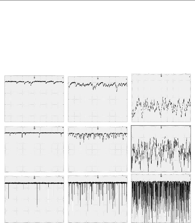
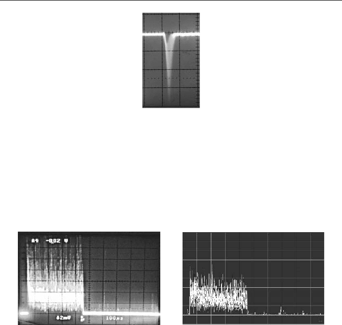
Fig. 1.1 Output signal of a photomultiplier tube at different light intensity and signal band-

width. Left to right: Average output current –1 uA, –10 uA and –100 uA. Top to bottom:

Bandwidth 1 MHz, 10 MHz, and 100 MHz. Time scale 1 µs / div., XP2020 PMT at –2,000 V

Time-Domain Techniques versus Frequency-Domain Techniques

Time-domain techniques record the intensity of the signal as a function of time,

frequency-domain techniques record the phase and the amplitude of the signal as a

function of frequency. Time domain and frequency domain are connected via the

Fourier transform. Therefore, the time domain and the frequency domain are gener-

ally equivalent. However, this does not imply an equivalence between time-domain

and frequency-domain recording techniques or the instruments used for each. An

exhaustive comparison of the techniques is difficult and needs to include a number

of different electronic design principles and applications.

1 Optical Signal Recording 3

In the following we assume that a sample is to be characterised by an optical

probing technique. It is excited by a modulated or pulsed light source. The light

emitted by the sample is recorded, and typical sample parameters are derived from

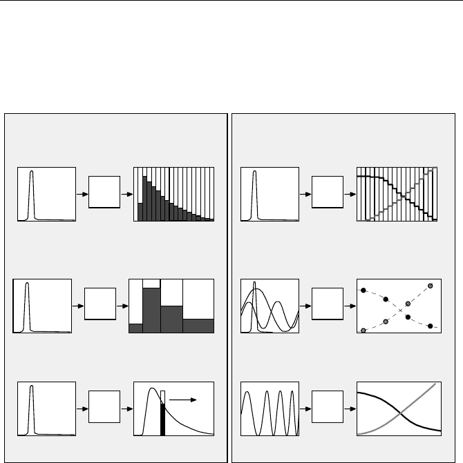
the recorded signal. Typical time-domain and frequency-domain techniques are

shown in Fig. 1.2.

Time Domain Frequency Domain

Sample

Pulsed Excitation

Simultaneous Recording

into many time channels

Sample

Pulsed Excitation

Pulse-by-Pulse Gate

Scan

Sample

Pulsed Excitation

Simultaneous Recording

into a few time channels

A) Digitizers, Multichannel Scalers, TCSPC

C) Multi-Gate Photon Counting

E) Boxcar Integrators, Gated Image Intensifiers

Sample

Pulsed Excitation

Simultaneous recording

of phase and amplitude

B) Technique does not exist

into many frequency channels

Sample

Pulsed or Sinewave

Excitation

Recording of amplitude and

phase, sequentially for a few

frequencies

D) Optical Modulation Techniques

Sample

Sinewave excitation

Frequency sweep

Amplitude and Phase

F) Electronic Network Analysers

Fig. 1.2 Time-domain (left) and frequency-domain techniques (right)

The most efficient way to record a signal in the time domain is to record its inten-

sity directly into a large number of time channels (A). For a sufficiently large num-

ber and sufficiently small width of the channels, the signal shape can be derived

from the data with a signal-to-noise ratio close to the ideal value, SNR = N

1/2

. A

number of recording techniques come close to the ideal, at least over a limited range

of signal intensity and time-channel width. Typical representatives are the time-

correlated single photon counting technique, the multichannel scaler technique,

and real-time digitising techniques.

The equivalent in the frequency domain is to excite the sample by light pulses

and to record the complete amplitude and phase spectrum at a large number of

frequencies simultaneously (B). Surprisingly, a useful technique for performing

this kind of measurement does not exist.

Often it is possible to model the behaviour of the sample or of the general

shape of the signal waveform or the signal spectrum. The number of time chan-

nels or the number of frequency channels into which the signal is recorded can

then be reduced. For example, fluorescence decay functions are weighted sums of

4 1 Optical Signal Recording

exponentials, which can be derived from only a few data points. A typical time-

domain technique of this group is multigate photon counting (C). The detected

photons are counted within a small number of subsequent time windows by sev-

eral parallel counters. The efficiency depends on the model of the sample and the

number and the width of the time gates. If a simple model is applicable to the

signal shape and the time gates are optimised for the expected sample parameters,

the efficiency can be almost ideal.

In the frequency domain, the sample is excited with modulated light (D). The

amplitude and the phase are measured at a single frequency or at a small number

of frequencies. Different modulation frequencies can be obtained by changing the

excitation frequency or by using different harmonics of a pulsed excitation wave-

form. The efficiency of the modulation technique depends on a number of techni-

cal details, especially the depth of modulation of the excitation light and the way

the detector signal is demodulated. Only for excitation with short pulses of high

repetition rate and ideal demodulation a near-ideal efficiency is obtained.

The signals can also be recorded sequentially (E and F). In the time domain, a

narrow time gate is scanned over the signal waveform (E). Gate scanning is used

in boxcar integrators, in gated photon counters, and in gated image intensifiers. Of

course, gate scanning yields a poor efficiency, because it gates off the majority of

the signal photons.

In the frequency domain, the frequency of the excitation is scanned, and the phase

and the amplitude are recorded as functions of the frequency (F). Frequency scanning

is used in electronic network analysers. The principle can be used for optical meas-

urements if the light source can be modulated electronically in a wide frequency

range. Differing from a gate scan in the time domain, the frequency scan technique

theoretically yields a near-ideal efficiency. However, in practice perfect efficiency

can be obtained only for excitation with short pulses, not for sinewave excitation.

Analog Techniques versus Photon Counting Techniques

There are two ways to interpret the detector signals shown in Fig. 1.1. The detec-

tor signal can be considered as a waveform superimposed over the shot noise of

the photons, or as a random sequence of pulses originating from individual pho-

tons. The first leads to analog signal recording, the second to photon counting.

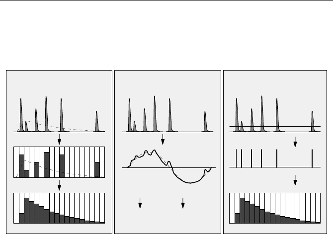
An analog technique based on direct digitising is shown in Fig. 1.3, left. The

detector signal is first digitised in short time intervals, and then accumulated over

a number of signal periods. Obviously, interpreting the detector signal as an ana-

log waveform causes problems at low intensities. The signal-to-noise ratio is the

square root of the number of photons, N, within the impulse response time of the

detector. At low intensity the signal-to-noise ratio drops far below 1. Eventually,

the detector signal becomes a sequence of a few, randomly spread pulses. The

frequency of the pulses can even drop far below one photon per signal period, in

which case baseline instability and electronic noise set a limit to the number of

accumulations and consequently to the sensitivity of the measurement. Obviously

analog recording is better suited to recording high-intensity signals.

The brute-force solution of time-domain analog recording is to use a low signal

repetition rate and a correspondingly higher laser peak power. The light intensity

1 Optical Signal Recording 5

within the pulses can then be increased without exceeding the maximum permissi-

ble average output current of the detector. However, pulsed operation at low duty

cycle and high intensity results in saturation effects in the sample, linearity errors

in the detector, and long-term degradation of detector performance.

Analog Recording - Time Domain Photon Counting

Detector Signal

Digitizing

Accumulation

Discrimination

Accumulation

Detector Signal

Analog Recording -

Detector Signal

Filtering

Phase-Sensitive Detection

Phase Amplitude

Time-Measurement

Frequency Domain

Fig. 1.3 Analog recording in the time domain (left), analog recording in the frequency

domain (middle), and photon counting (right)

Analog recording in the frequency domain is shown in Fig. 1.3, middle. The de-

tector signal is fed through a filter centred at the modulation (or pulse repetition)

frequency. The filter smoothes out the signal so that the random pulse sequence is

converted into a more or less noisy sinewave signal. The phase and amplitude of

this signal are measured by phase-sensitive detection. Baseline drift and low-

frequency noise are suppressed in the filter and do not cause many problems.

However, if the photon rate is so low that filtering does not yield a continuous

signal, reasonable phase information is no longer available. Therefore the effi-

ciency degrades at low photon rates.

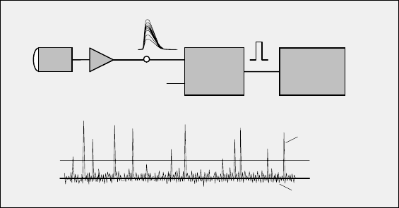
Photon counting is shown in Fig. 1.3, right. Each detector pulse represents the

detection of an individual photon. The pulse density of the signal, rather than the

signal amplitude, provides the measure of the light intensity at the input of the

detector. The pulses are detected by a discriminator. The output pulses of the dis-

criminator must be counted into a large number of time channels according to the

time in the signal period. This can be achieved by two different techniques. The

multichannel-scaler technique switches through the channels of a high-speed

memory and drops the discriminator pulses into the current memory channel.

Time-correlated single photon counting (TCSPC) measures the times of the indi-

vidual pulses and puts them into a channel labelled with the corresponding time.

The benefit of the TCSPC technique is that the time resolution of the recording is

not limited by the speed of the memory. The principle of TCSPC is described in

detail under Sect 2.4, page 20.

Photon counting, especially TCSPC, differs significantly from any analog tech-

nique in a number of important features, which will be discussed below.

6 1 Optical Signal Recording

Time Resolution and Signal Bandwidth

The signal bandwidth of an analog signal recording technique is limited by the

bandwidth of the detector. In other words, the width of the instrument response

function, or IRF, cannot be shorter than the width of the single electron response,

or SER, of the detector. The SER is the pulse that the detector delivers for a single

photoelectron, i.e. for a single detected photon.

The time resolution of photon counting is not limited by the SER width. In-

stead, it depends on the accuracy at which the arrival time of the individual pulses

can be determined. This accuracy is determined by the timing accuracy of the

discriminator at the input of the counting electronics, and by the transit time fluc-

tuations in the detector. The timing error can be an order of magnitude better than

the width of the SER. Therefore photon counting techniques yield a higher band-

width and a shorter IRF for a given detector than any analog recording technique.

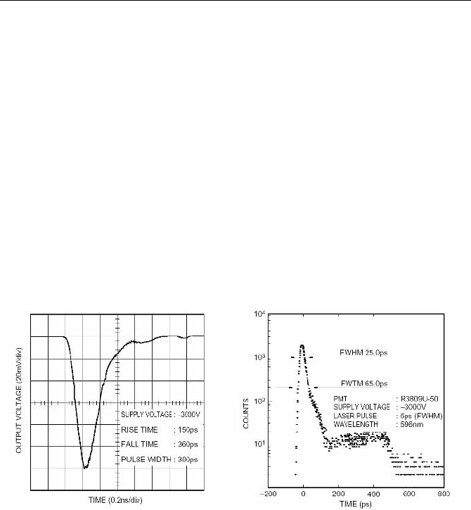
As an example, Fig. 1.4 shows the single-electron response measured with a

high-speed oscilloscope and the transit-time distribution for a Hamamatsu

R3809U MCP PMT measured by TCSPC.

Fig. 1.4 Single photon response (left) and transit-time distribution (right) of a Hamamatsu

R3809U MCP, from [211]

Although the width of the SER is 300 ps, the IRF width of the TCSPC meas-

urement is only 25 ps. The corresponding bandwidth is more than 10 GHz.

Please note: Bandwidth and IRF width should not be confused with the mini-

mum fluorescence lifetime detectable by a particular technique. The fluorescence

lifetime is obtained by fitting a model, in the simplest case an exponential func-

tion, to the recorded data. Depending on the signal-to-noise ratio of the raw data, a

lifetime considerably shorter than the IRF width can be measured.

Gain Noise

Due to the random nature of the amplification process in a photomultiplier tube or

avalanche photodiode, the single-photon pulses have a considerable amplitude jitter

(see Fig. 1.5). For analog processing, the amplitude jitter contributes to the noise

1 Optical Signal Recording 7

of the result. Photon counting techniques count all photons with the same weight.

The signal-to-noise ratio is not influenced by the gain noise of the detector.

An example is shown in Fig. 1.6. The same signal was recorded by an oscillo-

scope (left) and by photon counting (right). The counter binning time and the

oscilloscope risetime were adjusted to approximately the same value so that the

detection bandwidth was approximately the same. The lower SNR and the wider

noise amplitude distribution in the oscilloscope trace is clearly visible.

Fig. 1.6 Effect of amplitude jitter (gain noise) of the single-photon pulses of a PMT on the

recording of an optical pulse recorded by an analog oscilloscope (left) and by photon count-

ing (right)

Gain Stability

The gain of typical high-sensitivity detectors, e.g. photomultiplier tubes (PMTs) or

avalanche photodiodes (APDs), depends strongly on the supply voltage. It also

changes by degradation effects and ageing. For analog processing the magnitude

of the recorded signal changes with the detector gain. Although the influence of

the detector gain on the result provides a simple means of gain control, it is a per-

manent source of long-term instability. Photon counting directly delivers the num-

ber of photons per time interval. Within reasonable limits, the detector gain and its

instability have only negligible influence on the result.

Sample Rate

The sample rate, i.e. the density of the signal points on the recorded curves, must

by higher than twice the frequency of the fastest signal component present in the

Fig. 1.5 Amplitude jitter of the single-photon pulses of a PMT

8 1 Optical Signal Recording

signal. This relationship is known as the „Nyquist condition“. Only if the Nyquist

condition is fulfilled can the signal parameters be recovered without presumptions

about the signal shape. Time-domain analog recording techniques for sample rates

above a few GHz are inefficient, inaccurate, or extremely expensive.

If photon counting is used, the detection time of the individual photons can be

measured with a channel resolution of a few picoseconds, and can be used to build

up the photon distribution versus time. Time-correlated single photon counting

yields a time channel width of less that 1 ps, or an effective sample rate of more

than 1 THz.

Noise Rejection

As shown in Fig. 1.1, the detector signal at low light intensity is a random se-

quence of single-photon pulses. The average distance between the pulses can be

much longer than the pulse width. The signal can then only be recovered by ac-

cumulating a large number of signal periods. However, an analog technique also

accumulates the electronic noise floor and the baseline drift in the long gaps be-

tween the photons. Therefore the signal-to-noise ratio of all analog techniques

drops below the ideal value of N

1/2

at low light intensity.

Photon counting is insensitive to baseline drift and noise as long as the noise

and amplitudes are small compared to the amplitude of the single-photon pulses.

Therefore, the signal-to-noise ratio of photon counting techniques follows the N

1/2

law down to the detector background count rate.

Count Rate

The benefit of the analog recording techniques is that they can be used up to ex-

tremely high photon rates. If the detector gain can be reduced so that the detector

is not overloaded (i.e. does not start to respond nonlinearly and is not in danger of

damage), the detectable photon rate is virtually unlimited. This is, of course, not

so for photon counting techniques. Photon counting requires that the individual

photons remain distinguishable in the detector signal. This requires high detector

gain. Moreover, the average time intervals between the photon pulses must remain

considerably larger than the SER pulse width. Fast multichannel scalers in con-

junction with fast detectors work at peak count rates of several hundreds of MHz.

For continuous operation, the maximum permissible detector current limits the

count rates to a few tens of MHz.

Time-correlated single photon counting (TCSPC) measures the time of each in-

dividual photon. This is a relatively complicated operation, with a correspondingly

long signal processing time or „dead time“. Moreover, load-induced changes of

the detector response which remain unnoticed in other techniques show up in

high-resolution TCSPC results. Both the dead time and the stability of the detector

response set a limit to the count rate of TCSPC. Nevertheless, advanced TCSPC

devices can be operated up to count rates of several million photons per second

without noticeable loss in efficiency or accuracy.

1 Optical Signal Recording 9

Acquisition Time

It is often believed that analog techniques, in particular frequency-domain tech-

niques, are faster than photon counting techniques in terms of acquisition time.

Photon counting is usually considered to be a technique that delivers extremely high

time resolution, but also requires extremely long acquisition times. Certainly, ana-

log techniques have a virtually unlimited photon detection rate and are therefore

able to deliver short acquisition times at high intensities. On the other hand, early

photon counters, in particular TCSPC systems, had a very limited photon count

rate due to slow signal processing electronics. Moreover, they were hampered by

the low pulse repetition rate and low intensity of light sources of that time.

A closer look at the technical principles of TCSPC and their application to ex-

periments beyond the traditional fluorescence lifetime measurements reveals quite

a different picture now.

It has been mentioned above that the efficiency of TCSPC is near-ideal over a

wide range of sample-response times and intensities. As will be shown, advanced

TCSPC is also able to record in several detection channels simultaneously. If a

signal has to be resolved not only in time but also in wavelength, spatial coordi-

nates, or polarisation, the multidetector capability yields an enormous increase in

efficiency. As long as the detected photon rate does not exceed the counting capa-

bility of the TCSPC device, the acquisition time can be considerably shorter than

for any analog recording technique.

For example, optical detection techniques are increasingly used for experiments

on biological samples. The limited photostability of these samples sets severe

limitations to the excitation power. The photon rates obtained from most biologi-

cal samples are well within the counting capability of advanced TCSPC. Under

these conditions TCSPC yields acquisition times shorter than any analog tech-

nique.

Biological samples often show transient fluorescence effects. To investigate

these effects, either the amplitude and phase or the waveform of the signal have to

be acquired at intervals faster than the time scale of the changes. Frequency do-

main techniques are limited by the response time of the filters in the signal path,

and by the sequential recording of the amplitude and phase at different frequen-

cies. Photon counting can perform a fast sequence of consecutive measurements,

in acquisition time intervals of any length greater than the excitation period. It will

be shown that TCSPC is even able to deliver information about the detection time,

wavelength and polarisation of individual photons in the detected signal. The

recording of individual photons entirely wipes out the border between the resolu-

tion within a particular recorded waveform and consecutive waveforms. It opens

the way to a large number of experiments entirely beyond the reach of the cur-

rently known frequency-domain techniques. Spectroscopy of single molecules,

either freely diffusing or fixed in a substrate, can be performed on the microsec-

ond and millisecond time scale. It is not even necessary that the excitation light be

pulsed. Correlation between subsequent photons can be obtained by means of

continuous excitation and can be used to reveal diffusion, rotation, and conforma-

tional dynamics of single molecules and dye-protein complexes on any time scale

from picoseconds to milliseconds.

2 Overview of Photon Counting Techniques

2.1 Steady-State Photon Counting

The simplest photon counter consists of a detector, followed by a discriminator

and a counter (Fig. 2.1). The discriminator receives single-photon pulses from the

detector. To obtain pulses of sufficient amplitude at the discriminator input a pre-

amplifier can, but need not, be used in front of the discriminator.

Detector

Discrimi-

nator

Preamplifier

Counter

Threshold

Discriminator

threshold

Noise

Photon pulses

Photon

pulses

Fig. 2.1 Steady-state photon counter

The single-photon pulses have a more or less random amplitude. There is a

noise background consisting of low amplitude pulses from the detector, noise from

the environment, and electronic noise from the amplifier. The discriminator there-

fore has an adjustable threshold, which is set to discriminate the single-photon

pulses against the background noise. The discriminator threshold is set well above

the noise level, but below the peak amplitude of the photon pulses delivered by the

detector. When a single-photon pulse exceeds the selected threshold, the discrimi-

nator delivers a pulse of a defined duration and a defined logic level. The dis-

criminator output pulses are counted by the subsequent counter. The photons are

acquired for a given time interval, after which the result is read from the counter.

Although the simple circuit shown in Fig. 2.1 lacks any appreciable time reso-

lution, it has most of the positive features of photon counting: background sup-

pression, suppression of detector gain noise, and a sensitivity independent of de-

tector gain variations over a wide range. Photon counters of this type are often

12 2 Overview of Photon Counting Techniques

built as compact modules that include a detector, its power supply, a discrimina-

tor, a counter, and an RS 232 interface.

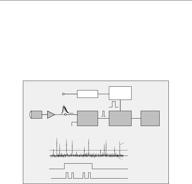
2.2 Gated Photon Counting

By adding a logic gate between the discriminator and the counter, single-photon

pulses can be counted within narrow time intervals. The principle is shown in

Fig. 2.2.

Detector

Discrimi-

nator

Preamplifier

Gate

Counter

Gate

Generator

Reference

Trigger /

Threshold

Discriminator

threshold

Noise

Photon pulses

Gate pulse

Pulses to counter

Gate Pulse

Photon pulses

Delay

Fig. 2.2 Gated Photon Counting

A discriminator separates the single-photon pulses from the background noise.

The discriminator output pulses are sent through a logic gate, and only pulses

within the gate pulse are counted. The gate pulses are triggered externally, e.g. by

a photodiode receiving the pulses of the excitation laser. Often a gate pulse gen-

erator and a delay generator are used to control the gate pulse duration and delay.

However, often the photons need to be counted only in a narrow, fixed time inter-

val within the signal pulse period. In these cases it is sufficient to derive a gate

pulse from the laser pulse via a fast photodiode and a discriminator [5, 27].

In practice the gate is often combined with the first counter stage. The principle

is shown in Fig. 2.3. Although this figure is somewhat technical, it is essential to

fully understand gated photon counting.