Astakhov V. Tribology of Metal Cutting

Generalized Model of Chip Formation 47

(a)

(b) (b)

100 µm

Fig. 1.31. Structures of the chip produced during machining of work material 3 at (a) ν =

150 m/min and (b) ν = 1500 m/min (Courtesy of Prof. S. Ekinovi

c).

appearance. As clearly seen in micrograph 6 in Figs. 1.28(c) and 1.31(b), the structure of

the chip obtained is similar to the continuous fragmentary humpback chip. A SEM image

of the free side of this chip (Fig. 1.31(c)) reveals the presence of the fragments and their

connectors.

Figure 1.28(d) shows the transformation of the chip structure with the cutting speed

for work material 4 (high-carbon steel, tempered). The structure of the chip produced

during machining with a cutting speed of ν = 50 m/min (micrograph 7 in Fig. 1.28(d))

belongs to the classical continuous fragmentary chip similar to that shown in Fig. 1.28(a).

Increasing the cutting speed to ν = 150 m/min (micrograph 8) leads to the onset of

unstable chip formation with low frequency f

= 3.84 kHz (the concept of frequency

of chip formation is explained later in this chapter). Relatively low temperature causes

the formation of almost separate chip fragments having relatively low strength of their

connectors. Further increasing the cutting speed to ν = 300 m/min does not change the

structure of the chip while resulting in higher chip formation frequency f

= 15.6 kHz

(micrograph 9 in Fig. 1.28(d)). As such, the strength of the chip connectors increases.

Even further increase in the cutting speed to ν = 1500 m/min does not change the

48 Tribology of Metal Cutting

structure of the chip while resulting in higher chip formation frequency f

= 100.6 kHz

(micrograph 10 in Fig. 1.28(d)).

Similar inﬂuence of the cutting speed on the chip structure and chip compression ratio

was revealed in the experiments conducted by Tónshoff et al. [95]. In their experiments,

much greater cutting speeds (up to 4000 m/min), different tool and work materials were

used. Comparison of their results with those presented in Fig. 1.28 reveals that the

frequency of chip formation (segmentation) depends both on the cutting speed and work

material. It is pointed out in both the studies that when chip distinctive segmentation is

the case (i.e. unstable chip formation takes place according to our current consideration),

the hardness of the border of a chip segment is severely deformed compared to the center

of this fragment.

1.7 Formation of Saw-Toothed Chip

Normally, when the work material is very ductile, there is always a great spread between

its ultimate tensile, σ

UTS

and yield tensile, σ

strengths. For example, AISI steel 303 has

the following characteristics: σ

UTS

= 620 MPa and σ

= 320 MPa while cold drawn

AISI steel 1045 has σ

UTS

= 625 MPa and σ

= 530 MPa. Moreover, some ductile

materials are characterized by a great dependence of their strength on temperature. When

such a material is machined, the saw-toothed chip is normally produced. This type of

chip is a particular case of the continuous fragmentary chip, where the size of “tooth”

becomes noticeable.

Talantov [96] was probably the ﬁrst to prove that thermodynamic equilibrium in the

deformation zone governs the chip formation process for the temperature-sensitive ductile

work materials. He suggested that the position of the shear plane changes during a chip

formation cycle in order to maintain this equilibrium during plastic deformation of the

chip on its formation. He also noticed that the grain structure of the chip varies over a

chip formation cycle.

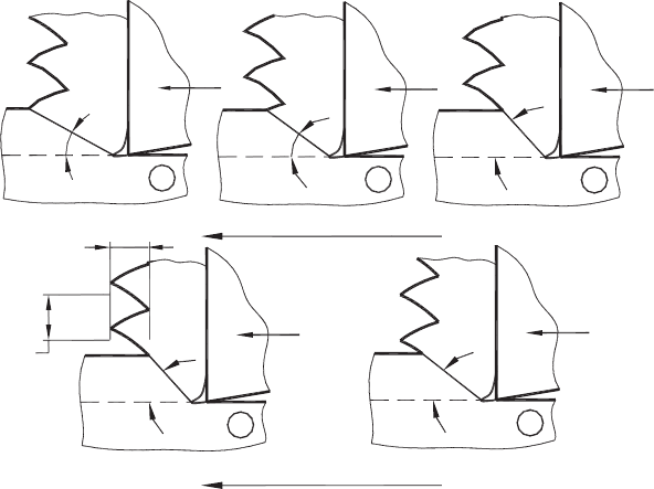
Figure 1.32 illustrates a cycle of chip formation of chip fragment B of the saw-toothed

continuous fragmentary chip. There are four distinctive phases in this cycle:

• Phase 1 is the initial stage of the cycle considered, where chip fragment A just

ﬁnished its formation. The surface of the maximum combined stress, approximated

by straight line ab, is located at an angle ϕ

max

with respect to the direction of the

cutting speed.

• Phase 2 is the beginning of the formation of fragment B. Due to the combined

action of the compressive and bending stresses and due to plastic deformation, the

inclination of the surface of maximum combined stress decreases. As such, this

surface is located at a certain intermediate angle ϕ

int1

. The temperature of the chip

formation zone increases as a direct result of plastic deformation.

• Phase 3 concludes the ﬁrst stage of plastic deformation of fragment B. During this

ﬁrst stage (Phases 1–3) fragment B is subjected to severe plastic deformation due to

great spread between the ultimate tensile, σ

UTS

and yield tensile, σ

strengths of

Generalized Model of Chip Formation 49

System Time

min

int1

max

int2

Fig. 1.32. System consideration of the model of chip formation of the saw-toothed continuous

fragmentary chip.

the work material. The amount of plastic deformation gained at the end of Phase 3 is

maximized so the resistance of the work material is the greatest due to its maximum

strain hardening. As a result, the inclination of the surface of maximum combined

stress is minimum which is thus characterized by the angle ϕ

min

. As a result of

severe plastic deformation of partially formed chip fragment B, the temperature

in the deformation zone increases to its maximum at this stage. This temperature

lowers the resistance of the work material.

• Phase 4 shows an intermediate stage of the second stage of the formation of chip

fragment B where the surface is located at a certain intermediate angle ϕ

int2

. The

amount of plastic deformation gained by this chip fragment decreases as this angle

increases. This phase eventually leads to Phase 5 (which is the same as Phase 1),

where the chip fragment B just ﬁnished its formation. The surface of the maximum

combined stress, approximated by straight line ab, is again located at angle ϕ

max

with respect to the direction of the cutting speed. The temperature due to plastic

deformation is at a minimum at this stage. Then a new cycle begins.

The pitch of the chip, p

and the depth of the chip proﬁle, t

depend on the properties

of the work material (spread between its ultimate and yield tensile strengths under a

given state of stress in the deformation zone; dependence of its strength on temperature;

toughness, which deﬁnes the energy spent in its plastic deformation), on the machining

regime (the pitch depends on the cutting speed while the proﬁle depth depends on the

cutting feed (uncut chip thickness)) and on the tool geometry (the normal rake and

inclination angles), which deﬁne the state of stress in the deformation zone.

50 Tribology of Metal Cutting

Figure 1.33 shows the results of FEM modeling for the case considered. The following

conditions were considered in this modeling:

• Tool: normal rake angle γ

= 0

◦

, normal ﬂank angle α

= 7

◦

, inclination angle

= 0

◦

, radius of the cutting edge ρ

= 0.005 mm, tool material is K15.

• Work material: AISI steel 316L, σ

UTS

= 517 MPa and σ

= 218 MPa.

• Cutting regime: cutting speed ν = 75 m/min, uncut chip thickness t

= 0.2mm,

width of cut d

= 2 mm.

Figures 1.33(a) and (b) show the state of the deformation zone for Phases 3 and 5,

respectively. As shown, these results correspond to the model shown in Fig. 1.32.

Figures 1.33(c) and (d) show the temperature distribution in the deformation zone

for these two stages. These results correspond to the model description showing the

above-described temperature variation in the deformation zone. Figures 1.33(e) and

(f) present the stress distribution in the deformation zone for the phases discussed.

Therefore, these FEM results fully support the described physical model of saw-toothed

chip formation.

To verify the discussed model experimentally, a series of cutting tests were carried

out. The following work materials were used in the tests: (a) AISI steel 1045 HR

ASTM A576 RD, and (b) AISI stainless steel 303 ANN CF RD ASTM A582 93. The

composition, element limits and deoxidation practice were chosen to comply with the

requirements of standard ANSI/ASME B94.55M-1985. To simulate the true orthogonal

cutting conditions, the special specimens were used [25]. After being machined to

the conﬁguration, the specimens were tempered at 180–200

◦

C to remove the residual

stresses. The hardness of each specimen has been determined over the whole working

part. Cutting tests were conducted only on the specimens where the hardness was within

the limits of ± 10%. Special parameters of the microstructure of these specimens such as

the grain size, inclusions count, etc. was determined for the initial workpiece structures

(shown in Figs. 1.34(a) and 1.35(a)) using quantitative metallography. The samples of

the chip, obtained in cutting experiments, are shown in Figs. 1.34(b) and 1.35(b).

The chip structure shown in Fig. 1.34(b) is a typical structure of continuous fragmentary

chip obtained in the machining of ductile materials, the strength of which has low sensi-

tivity to temperature. Very ﬁne, irregular and heavy deformed (the microhardness of the

chip is almost two times higher (285 HV) than that of the original material (163 HV))

“teeth” are formed on the chip free surface when this kind of steels are not pre-hardened

or modiﬁed to low or high alloys. A similar structure is shown in Fig. 1.28 for work

material 1. As shown from this ﬁgure, a signiﬁcant increase in the cutting speed leads

to coarsening of the “teeth” on the chip free surface due to high temperature involved in

the chip formation.

The chip structure shown in Fig. 1.35(b) is a typical saw-toothed continuous fragmentary

chip. To support the explanations given to the model shown in Fig. 1.32, the variation

of plastic deformation during a chip formation cycle should be clearly shown. As such,

higher plastic deformation should be the case during the loading stage of a cycle (Phases

2 and 3 in Fig. 1.32) and lower plastic deformation during the unloading stage of this

Generalized Model of Chip Formation 51

(a)

(b)

X 400

X 200

Fig. 1.34. Work material – AISI 1045 steel. Micrographs of (a) the initial structure and (b) the

chip structure obtained in orthogonal cutting test with a cutting speed of 60 m/min, equivalent

cutting feed of 0.2 mm/rev. Etched with 10 ml Nital and 90 ml alcohol (after Astakhov [18]).

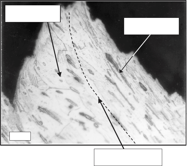
cycle (Phases 4 and 5 in Fig. 1.32). Figure 1.36 shows a fragment of the saw-toothed

chip shown in Fig. 1.35(b). As clearly shown, the deformed structure of this fragment

consists of two distinctive zones: zone of high plastic deformation where the grains are

severely deformed and zone of low plastic deformation where the grains are moderately

deformed.

The visual observations discussed may be subjective. To overcome these difﬁculties,

two-dimensional microhardness maps of the chips were taken to map out different zones

through the chip section. As discussed in [25], microhardness is uniquely related to

52 Tribology of Metal Cutting

(a)

(b)

X 400

X 150

Fig. 1.35. Work material – AISI 303 stainless steel. Micrographs of (a) the initial structure and

(b) the chip structure obtained in orthogonal cutting test with cutting speed of 60 m/min, equivalent

cutting feed of 0.2 mm/rev. Etched with 40 ml hydroﬂuoric (HF), 20 ml nitric acid and 40 ml

glycerine (After Astakhov [18]).

the plastic strain of a deformed body as well as to the shear stress gained at the last

stage of deformation. In this study, a Leco M400-G2 microhardness tester was used.

This machine operates by automatically indenting the specimen over an area deﬁned

by a grid of measurement points. At each location, indentation depth and load are

measured as the load is applied. Microhardness was determined using the principles

outlined in ISO standard for Instrumented Hardness Tests, ISO DIS 14577. The posi-

tion of the surface is identiﬁed by ﬁtting a polynomial to the initial 5% of the loading

curve.

Generalized Model of Chip Formation 53

X600

Zone of low plastic

deformation

Zone of high plastic

deformation

Conditional boundary

between two zones

Fig. 1.36. A chip fragment of the chip shown in Fig. 1.36(b).

The displacement at maximum load incorporates elastic and plastic deformation. A linear

ﬁt to the top 20% of the unloading curve (representing elastic unloading) is extrapolated to

zero load to determine the depth of the material in contact with the indenter at maximum

load. The test results show that for the chip fragment shown in Fig. 1.36, average

microhardness in the zone of high plastic deformation is 335 HV while that in the zone

of low plastic deformation is 225 HV. These results conclusively prove the adequacy of

the model of saw-toothed chip formation shown in Fig. 1.32.

1.8 Frequency of Chip Formation

As the chip formation process appears to be cyclic, its frequency is of interest. The fre-

quency of chip formation can be measured by calculating the number of teeth produced

in unit time as proposed by Talantov [96]. However, there are two drawbacks in this

method. First, the pitch of the saw-tooth chip (p

in Fig. 1.32) is not always easy to

measure because a lengthy mounting process is required. The accuracy of the evalua-

tion is not high because the pitch may vary (for example, due to the variation in the

microstructure of the work material) over the length of the chip and thus a rather long

chip should be taken into evaluation, which may not be feasible. If only a short chip

fragment (for example as shown in Fig. 1.37) were considered, the averaging of p

would not guarantee correct results. Second, it is not applicable for the analysis of the

54 Tribology of Metal Cutting

X100

Fig. 1.37. Quick-stop micrograph of a partially formed chip. Work material is AISI steel 4140.

Cutting conditions: cutting speed ν = 85 m/min, feed f = 0.14 mm/rev, rake angle γ

= 12

◦

ﬂank angle α

= 10

◦

. Orthogonal dry cutting.

continuous fragmentary chip when the depth of proﬁle t

(Fig. 1.32) is very small as,

for example, the chip shown in Fig. 1.34.

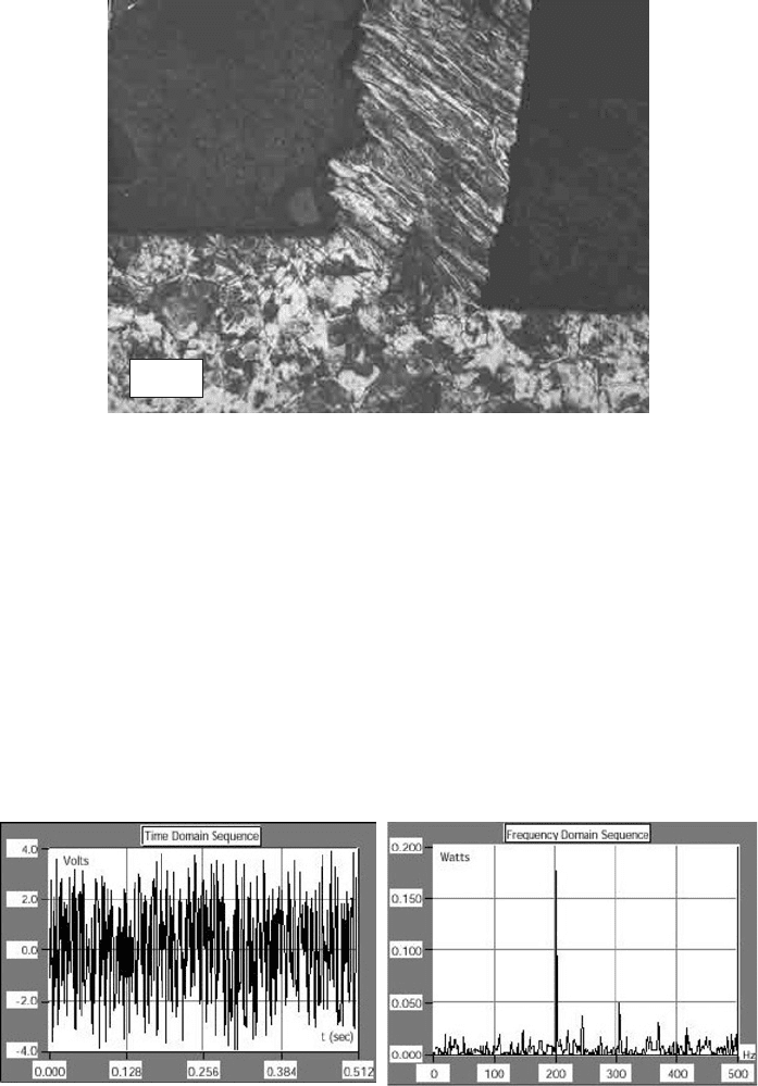
Lindberg and Lindstrom [97] proposed direct measurement of this frequency using a

digital spectrum analyzer. One common method of visualizing a dynamometer signal

is in the time domain (Fig. 1.38(a)). This representation often plots the signal value

(commonly a voltage or current that represents the measurement of force, temperature or

strain) as a function of time. Another useful signal representation is the frequency-domain

view of the signal (Fig. 1.38(b)). This representation is typically based on a variation of

(a)

(b)

Fig. 1.38. Cutting force signal in the time domain (a) and its representation in the frequency

domain (b) obtained using LabView FFT by National Instruments Co.

Generalized Model of Chip Formation 55

the Fourier Transform and commonly plots the frequency or phase content of a signal as

a function of frequency. By examining the frequency-domain view of the signal, useful

information about the measured signal can be derived that might not be immediately

apparent from an examination of the time-domain representation. For a given signal,

the power spectrum gives a plot of the portion of a signal’s power (energy per unit

time) falling within given frequency bins. The most common way of generating a power

spectrum is by using a discrete Fourier transform [98]. It can be accomplished using a

digital spectrum analyzer [25,97].

Figures 1.39(a)–(c) show the examples of the results of a study of the chip formation

frequency of different work materials (the test methodology is discussed in detail in

[99]). These ﬁgures show the frequency power spectra of cutting force obtained in the

machining of different materials at the same cutting regimes and dimensions of the work-

pieces. As shown, the dynamic response of the machining system, including machine

tool, depends not only on the system’s geometry and cutting regime used, but also on

a particular workpiece material used. The results of this study reveal that the frequency

of the chip formation process primarily depends on the cutting speed and on the work

material. The cutting feed and the depth of cut (>1 mm) have very small inﬂuence on

this frequency. The dependence of the chip formation frequency on the cutting speed was

obtained by taking power spectra similar to those shown in Figs. 1.39(a)–(c) at different

cutting speeds. The results are shown in Fig. 1.40.

The results obtained also show that when the dynamic experiments are conducted prop-

erly, i.e. when the noise (for example, due to the misalignment of the workpiece and

other machining system inaccuracies) is eliminated from the system response, the ampli-

tudes of peak at the frequency of chip formation are the largest in the corresponding

autospectra. Unfortunately, this fact is not considered in the dynamic analysis of the

machining systems where the cutting process as the main source of vibration is practically

ignored.

1.9 Formation of the Segmental Saw-Toothed Chip

The formation of the segmental saw-toothed chip similar to that shown in Fig. 1.28(d)

(micrographs 8–10) attracted the attention of some researchers due to wider use of high-

speed machining and a great number of difﬁcult-to-machine alloys. Shaw [45] claims

that he was the ﬁrst to publish a micrograph of the saw-toothed chip in 1954, obtained in

turning of a titanium alloy, when this work material was initially being considered as a

structural material. In this micrograph, presented by Shaw (Fig. 3(a) in [45]), however, no

severe plastic deformation can be observed in the regions adjacent to the cracks formed

between the chip elements. Actually, the same can be said about other micrographs

presented in this picture for continuous fragmentary chip where the heavily deformed

chip contact layer, normally found in this kind of the chip, is not seen.

Nakayama studied the metal cutting process using a highly cold-worked brass as the

work material at very low cutting speeds and suggested [100] a theory of saw-toothed

chip formation. The model used to describe this theory is shown in Fig. 1.41(a).

56 Tribology of Metal Cutting

−120

−100

−80

−60

−40

−20

−120

−100

−80

−60

−40

−20

−120

−100

−80

−60

−40

−20

0 200 400 600 800 1000 1200 1400 1600 1800

Frequency (Hz)

Cutting force (db ref 5000N)

Feed f = 0.12 mm/rev

Frequency (Hz)

Cutting force (db ref 5000N) Cutting force (db ref 5000N)

Feed f = 0.12 mm/rev

Frequency (Hz)

(a)

(b)

(c)

Fig. 1.39. Power spectra for the cutting force signal. Work materials: (a) AISI steel 303, (b) AISI

steel 4340 and (c) AISI steel 1045 (after Astakhov [25]).

Astakhov V. Tribology of Metal Cutting

Подождите немного. Документ загружается.