ASM Metals HandBook Vol. 17 - Nondestructive Evaluation and Quality Control
Подождите немного. Документ загружается.

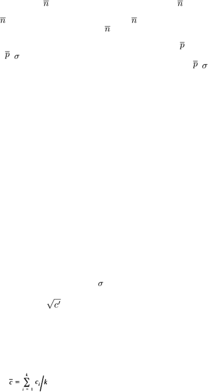
100% inspection) and production rates vary from day to day. Because the limits on a p-chart depend on the sample size n,
some adjustments must be made to ensure that the chart is properly interpreted. There are several ways in which the
variable sample size problem can be handled. Some of the more common approaches are the following:
• Compute separate limits for each individual subgroup. This approach certainly
leads to a correct set of
limits for each sample, but requires continual calculation of the control limits and a somewhat messy-
looking control chart
• Determine an average sample size, , and a single set of control limits based on
. This method may be
appropriate if the sample sizes do
not vary greatly, perhaps no more than about 20%. However, if the
actual n is less than , a point above the control limit based on
may not be above its own true upper
control limit. Conversely, if the actual n is greater than
, a point may not show out of control when in
reality it is
• A third procedure for varying sampling size is to express the fraction defective
in standard deviation
units, that is, plot (p - )/
p
on a control chart where the centerline is zero and the control limits are set
at ±3.0. This stabilizes the plotted value even though n may be varying. Note that (p - )/
p
is a familiar
form; recall the standard normal (Z
) distribution. For this method, the continued calculation of the
stabilized variable is somewhat tedious, but the chart has a clean appearance, with constant limits of
always ±3.0 and constant centerline at 0.0
c-Chart: A Control Chart for Number of Defects
The p-chart deals with the notion of a defective part or item where defective means that the part has at least one
nonconformity or disqualifying defect. It must be recognized, however, that the incidence of any one of several possible
nonconformities would qualify a part for defective status. A part with ten defects, any one of which makes it a defective,
is on equal footing with a part with only one defect in terms of being a defective.
Often it is of interest to note every occurrence of every type of defect on a part and to chart the number of defects per
sample. A sample may only be one part, particularly if interest is focusing on final inspection of an assembled product,
such as an automobile, a lift truck, or perhaps a washing machine. Inspection may focus on one type of defect (such as
nonconforming rivets on an aircraft wing) or multiple defects (such as flash, splay, voids, and knit lines on an injection-
molded truck grille).
Considering an assembled product such as a lift truck, the opportunity for the occurrence of a defect is quite large,
perhaps to be considered infinite. However, the probability occurrence of a defect in any one spot arbitrarily chosen is
probably very, very small. In this case, the probability law that governs the incidence of defects is known as the Poisson
law or Poisson probability distribution, where c is the number of defects per sample. It is important that the opportunity
space for defects to occur be constant from sample to sample. The Poisson distribution defines the probability of
observing c defects in a sample where c' is the average rate of occurrence of defects per sample.
Construction of c-Charts From Sample Data. The number of defects, c, arises probabilistically according to the
Poisson distribution. One important property of the Poisson distribution is that the mean and variance are the same value.
Then given c', the true average number of defects per sample, the 3 limits for the c-chart are given by:
CL
c
= c' ± 3
(Eq 5)
Note that the standard deviation of the observed quantity c is the square root of c'. The Poisson distribution is a very
simple probability model, being completely described by a single parameter c'.
When c' is unknown, it must be estimated from the data. For a collection of k samples, each with an observed number of
defects c, the estimate of c' is:
(Eq 6)
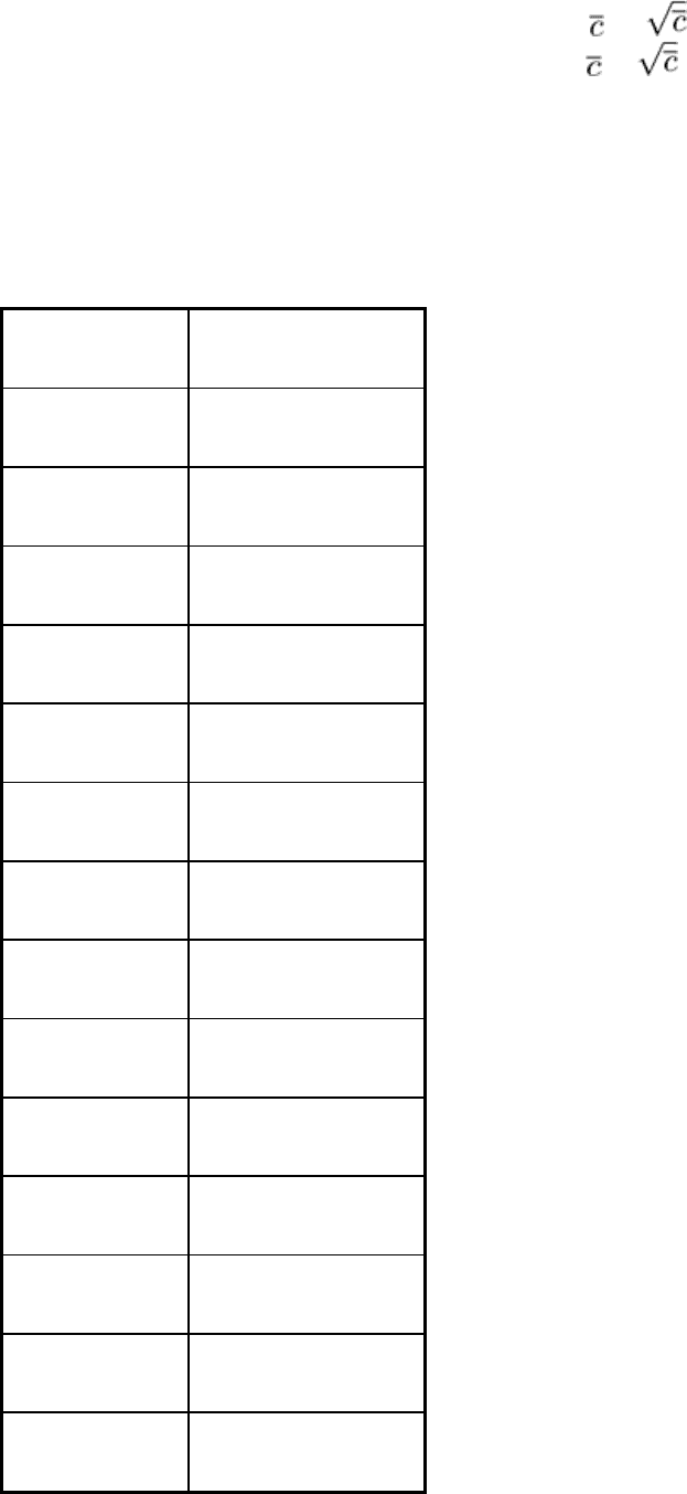
Therefore, trial control limits for the c-chart can be established, with possible truncation of the lower control limit at zero,
from:
UCL
c
= + 3
LCL
c
= - 3
Example 4: c-Chart Construction for Continuous Testing of Plastic-Insulated Wire at a
Specified Test Voltage.
Table 5 lists the results of continuous testing of a certain type of plastic-covered wire at a specified test voltage. This test
causes breakdowns at weak spots in the insulation, which are cut out before shipment.
Table 5 c-chart data for plastic-insulated wire of Example 4
Sample number, k
Number of breakdowns
1 1
2 1
3 3
4 7
5 8
6 1
7 2
8 6
9 1
10 1
11 10
12 5
13 0
14 19

15 16
16 20
17 1
18 6
19 12
20 4
21 5
22 1
23 8
24 7
25 9
26 2
27 3
28 14
29 6
30 8
The original data consisted of the number of breakdowns in successive lengths of 1000 ft each. There may be 0, 1, 2, 3, . .
., breakdowns per length, depending on the number of weak spots in the insulation. However, so few defects were
obtained during a short period of production by using the 1000 ft length as a unit and the expectancy in terms of the
number of breakdowns per length was so small that a longer length of 10,000 ft was used for the unit size for the
corresponding c-chart. In general, it is desirable to select the sample size for the c-chart application such that on average
( ) at least one or two defects are occurring per sample.
In most applications, the centerline of the c-chart is based on the estimate of the average number of defects per sample.
This estimate can be calculated by:
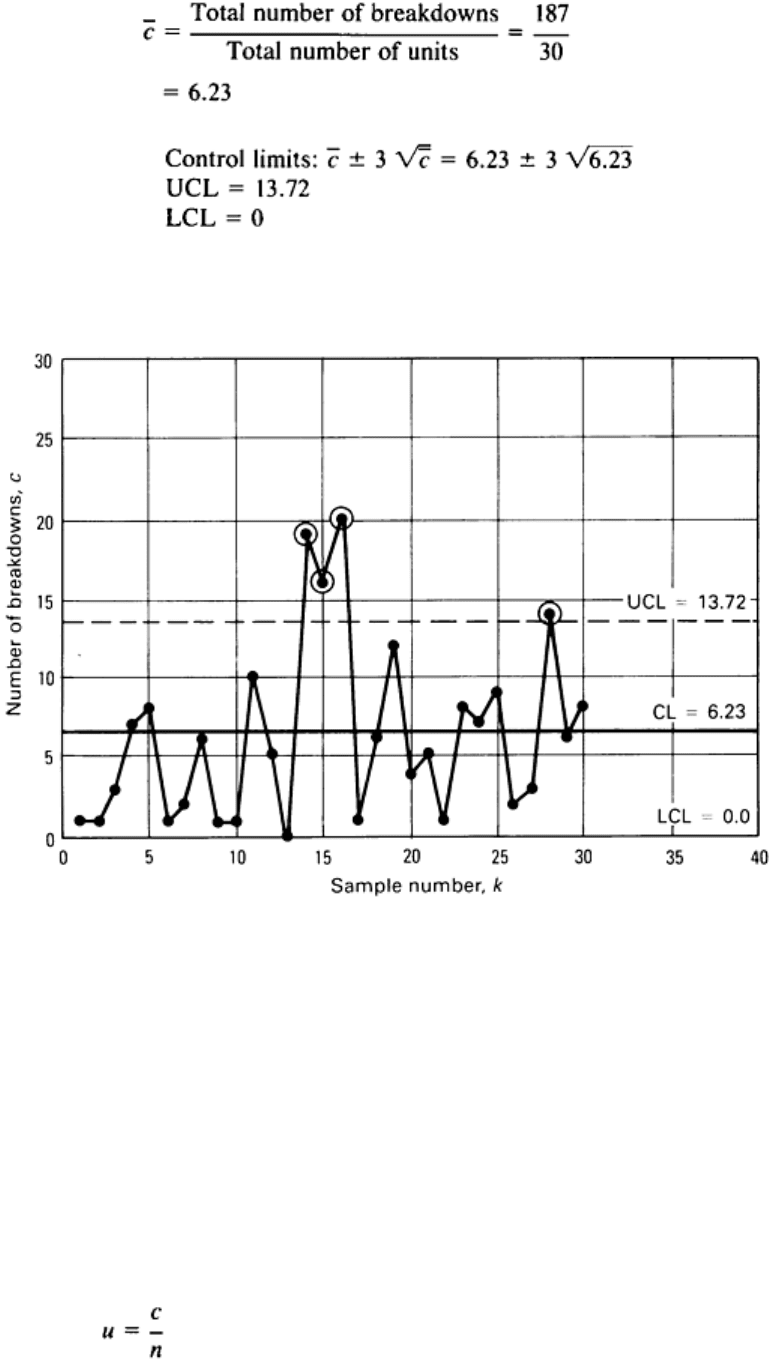
The resulting c-chart in Fig. 31 shows the presence of special causes of variation.
Fig. 31 c control chart obtained for the evaluation of the plastic-insulated wire data (k = 30) in Table 5
u-Chart: A Control Chart for the Number of Defects per Unit
Although in c-chart applications it is common for a sample to consist of only a single unit or item, the sample or subgroup
can be comprised of several units. Further, from subgroup to subgroup, the number of units per subgroup may vary,
particularly if a subgroup is an amount of production for the shift or day, for example.
In such cases, the opportunity space for the occurrence of defects per subgroup changes from subgroup to subgroup,
violating the equal opportunity space assumption on which the standard c-chart is based. Therefore, it is necessary to
create some standardized statistic, and such a statistic may be the average number of defects per unit or item where n is
the number of items per subgroup. The symbol u is often used to denote average number of defects per unit, that is:
(Eq 7)
where c is the total number of defects per subgroup of n units. For k such subgroups gathered, the centerline on the u-
chart is:
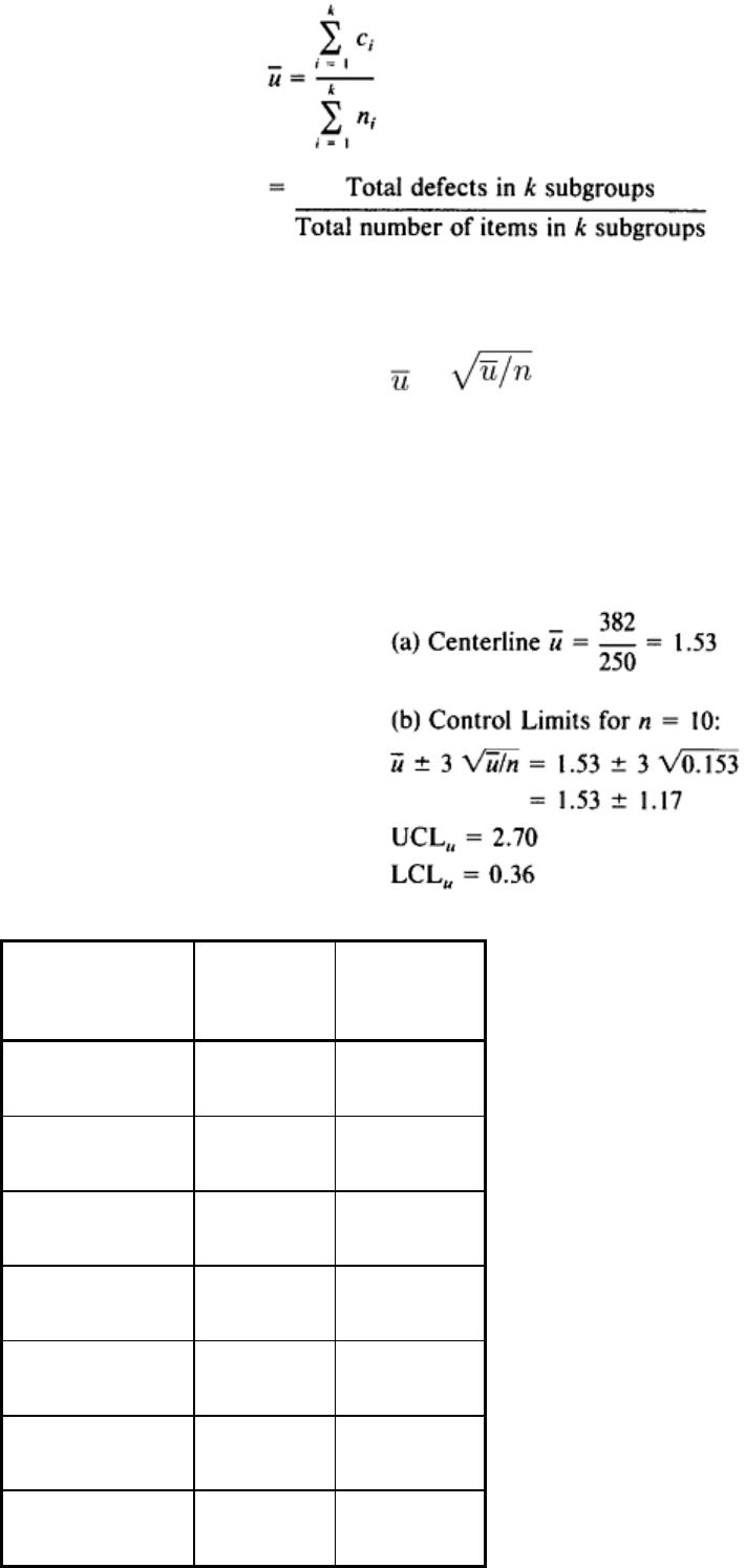
(Eq 8)
The trial control limits for the u-chart are then given by:
CL
u
= ± 3
(Eq 9)
Example 5: Use of the u-Chart to Evaluate Leather Handbag Lots.
Table 6 lists inspection results in terms of defects observed in the inspection of 25 consecutive lots of leather handbags.
Because the number of handbags in each lot was different, a constant sample size of n = 10 was used. All defects were
counted even though two or more defects of the same or different type occurred on the same bag. The u-chart data are as
follows (Fig. 32):
Table 6 u-chart data for leather handbag lot production of Example 5
Sample number, k
(a)
Total number
of defects
Defects per unit
1 17
1.7
2 14
1.4
3 6
0.6
4 23
2.3
5 5
0.5
6 7
0.7
7 10
1.0

8 19
1.9
9 29
2.9
10 18
1.8
11 18
1.8
12 5
0.5
13 8
0.8
14 11
1.1
15 18
1.8
16 13
1.3
17 22
2.2
18 6
0.6
19 23
2.3
20 22
2.2
21 9
0.9
22 15
1.5
23 20
2.0
23 20
2.0
25 24
2.4
Total 382 38.2
(a)
n = 10
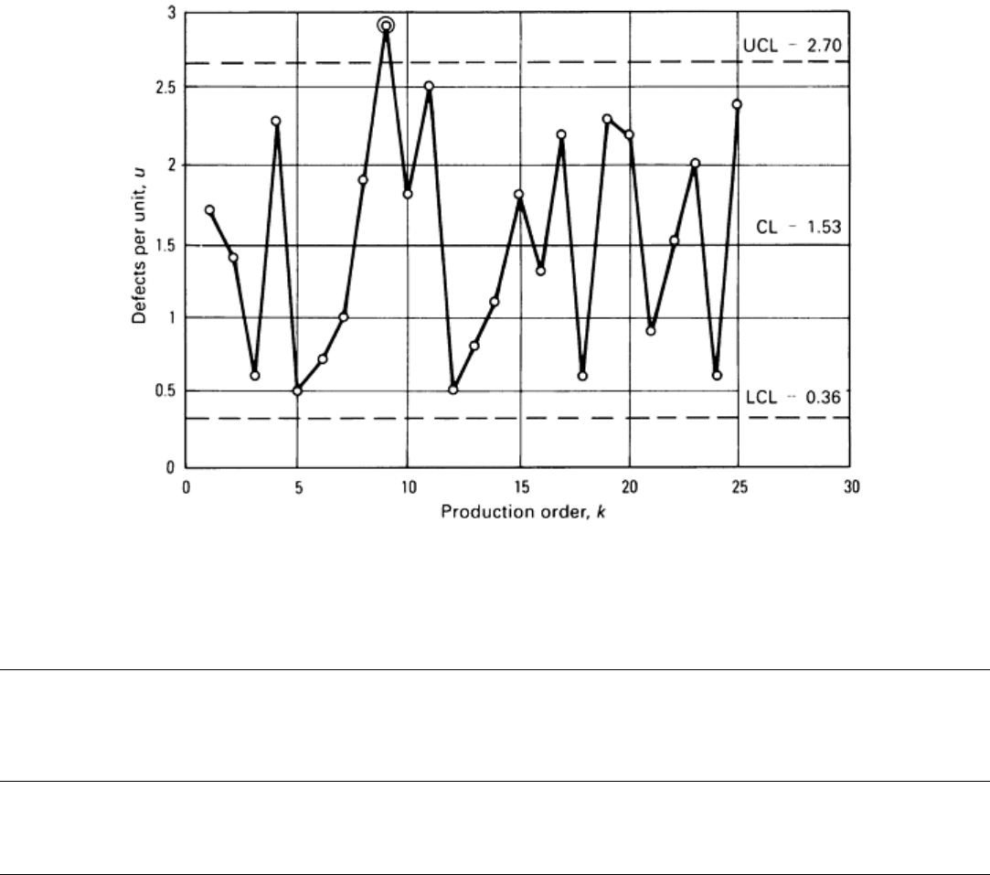
Fig. 32 u control chart obtained for the evaluation of leather handbag lot data in Table 6. Data are for k
= 25,
n = 10. Datum for sample 9 is an extreme point because it exceeds value of UCL.
Reference cited in this section
22.
I. Burr, Statistical Quality Control Methods, Marcel Dekker, 1976
Statistical Quality Design and Control
Richard E. DeVor, University of Illinois, Urbana-Champaign; Tsong-how Chang, University of Wisconsin, Milwaukee
Process Capability Assessment
This section presents both traditional and more modern views of process capability and how it is assessed. The
presentation stresses the relationship between the control/stability of a process and its capability. The clear distinction
between the engineering specification and the statistical control limits in terms of their use and interpretation is
emphasized. Using the traditional conformance to the specifications view of process capability, this section illustrates the
consequences of a lack of statistical control in terms of the manner and extent to which a process produces parts that meet
design intent. This section also presents the loss function approach to the articulation of process capability.
Process Capability Versus Process Control
There are two separate but vitally important issues that must be addressed when considering the statistical representation
of process data. These are:
• The ability of the process to produce parts that conform to specifications
• The ability of the process to maintain a state of good statistical control
These two process characteristics are linked in the sense that it will be difficult to assess process capability with respect to
conformance to specifications without being reasonably assured of having good statistical control. Although control
certainly does not imply conformance, it is a necessary prerequisite to the proper assessment of conformance.
In a statistical sense, conformance to specifications involves the process as a whole; therefore, attention will be focused
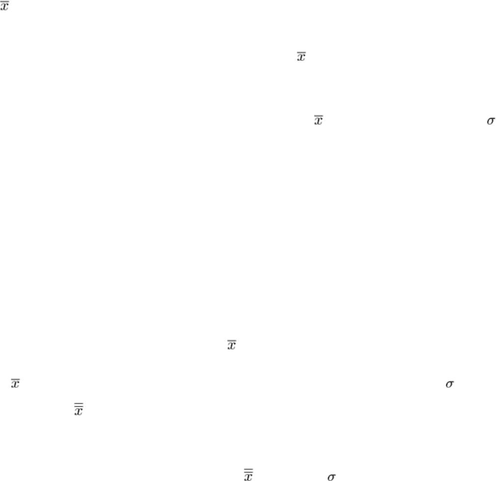
on the distribution of individual measurements. In dealing with statistical control, summary statistics from each sample,
mainly and R, are used; as a result, this involves the distribution of these statistics, not individual measurements.
Because of the above distinction between populations and samples, it is crucial not to compare or confuse part
specifications and control limits. In fact, tolerance/specification limits should never be placed on a control chart. This is
so because the control chart is based on the variation in the sample means , while it is the individual measurements in
the sample that should be compared to specifications. Placing specifications on the control chart may lead to the mistaken
impression that good conformance exists when, in fact, it does not. This is illustrated in Example 6.
A process may produce a large number of pieces that do not meet the specified production standards, even though the
process itself is in a state of good statistical control (that is, all the points on and R control charts are within the 3
limits and vary in a random manner). This may be because the process is not centered properly; in other words, the actual
mean value of the parts being produced may be significantly different from the specified nominal value of the part. If this
is the case, an adjustment of the machine to move the mean closer to the nominal value may solve the problem. Another
possible reason for lack of conformance to specifications is that a statistically stable process may be producing parts with
an unacceptably high level of common cause variation. In summary, if a process is in statistical control but not capable of
meeting the tolerances, the problem may be one of the following:
• The process is off-center from the nominal
• The process variability is too large relative to the tolerances
• The process is off-center and with large variation
Example 6: Statistical Assessment of Process Capability for a Workpiece.
For a certain part, a dimension of interest was specified by the engineering department as 0.140 ± 0.003 in. Many parts
were being rejected on 100% inspection using a go/no-go gage because they failed to meet these tolerances.
It was decided to study the capability of the process using and R control charts. These data were taken from the same
machine and operator and at the rate of about one sample per hour.
Both the and R control charts seem to indicate good statistical control with no points exceeding the 3 limits, a
reasonably normal distribution of points between the limits, and no discernible trends, cycles, and so on. Therefore, the
calculated sample mean = 0.1406 in. and the sample standard deviation σ
x
= 0.0037 in. are good estimates. The process
can then be evaluated with respect to its conformance to specifications.
To obtain a clear picture of the statistical nature of the data, a frequency histogram was plotted that resembled a normal
distribution, but the mean appears to be slightly higher than the nominal value of 0.140 set by the engineering department.
Figure 33 shows this population distribution curve centered at with a spread of
x
= 0.0037 in. The specifications are
also shown on this plot.
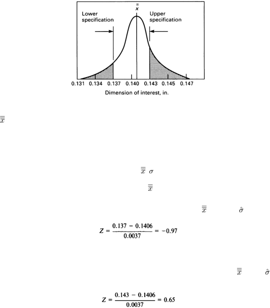
Fig. 33 Normal distribution model for process capability for the data of Example 6. LSL
x
= 0.137, USL
x
= 0.143,
= 0.1406, and σ
x
= 0.0037.
The shaded areas in Fig. 33 represent the probability of obtaining a part that does not meet specifications. To compute the
probability of a part failing below the lower specification, the standard normal distribution, Z, is calculated, and a normal
curve table is used:
Z = (x - )/
x
where x is the value of either the lower or upper specification, is the estimate for the population mean, and σ
x
is the
estimate of the process standard deviation.
To find the probability of a point below the lower specification limit, LSL
x
= 0.137, with = 0.1406, and
x
= 0.0037:
Looking this value up in the normal table produces Prob (0.137 or less) = 0.1660. This means that there is a 16.6% chance
of an individual part falling below the specified tolerance.
To find the probability of an individual part falling above the upper specification limit, USL
x
= 0.143, = 0.1406,
x
=
0.0037, and:
The probability of a part being above the upper specification limit is equal to 0.2578, based on Z = 0.65. The process that
does not meet the specifications is therefore 16.6% + 25.78% = 42.37%.
It might be asked whether centering the process at the nominal value of 0.140 would help. To check, a normal curve is
constructed, centered at 0.140. The probability of a point below the lower specification is found by computing Z using the
nominal value as the population mean:
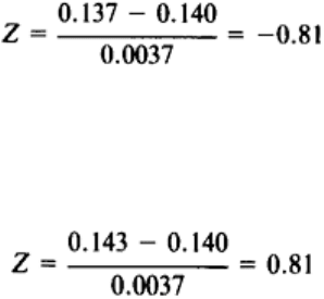
Looking up the area for this Z value in the normal curve table produces a value of 0.209, which is the probability of
getting a value below the lower specification limit. The probability of getting a value above the upper specification is
found by:
which from the normal curve table gives an area = 0.209. The total probability of a part not meeting specification is the
sum of these, or 0.209 + 0.209 = 0.41, or 41%.
Therefore, recentering the process will not be of much help. The process is in control; no special causes of variability
were indicated. However, about 42% of the parts were outside the tolerances. Possible remedies include the following:
• Continue to sort by 100% inspection
• Widen the tolerances, for example, 0.140 ± 0.006
• Use a more precise process; reduce process variation
• Use statistical methods to identify variation reduction opportunities for the existing process
Too often, the strategy used (or at least urged) is the second remedy listed above. Clearly, a stronger consideration should
be given to the final remedy listed above.
Comparison of Tolerances and Control Limits
It is important to clearly differentiate between specification limits and control limits. The specification limits or tolerances
of a part are:
• Characteristic of the part/item in question
• Based on functional considerations
• Related to/compared with an individual part measurement
• Used to establish the conformability of a part
The control limits on a control chart are:
• Characteristic of the process in question
• Based on process variability
• Dependent on sampling parameters, namely, sample size
• Used to identify presence/absence of special cause variation in the process
Control limits and tolerances must never be compared numerically and should not appear together on the same graph.
Tolerances are limits on individual measurements and as such can be compared against the process as a whole as
represented by many individual measurements collected in the form of a statistical distribution, as was done in Example 6
to assess overall process capability.
Process Capability Indices
It is common to measure process capability in the units of process standard deviations. In particular, it is common to look
at the relationship between the process standard deviation and the distance between the upper and lower specification:
